How to overlay shapefile data on PyGMT Maps

PyGMT library in Python made plotting high-resolution topographic maps a breeze. It comes packaged with shorelines, country borders and topographic data. Often, we need to highlight an arbitrarily selected polygon shapes or region on a map using available shapefile data.

In this post, we will see how we can overlay shapefile data on top of the PyGMT map using geopandas library. Here, for example, I obtained the counties data available in .shp format from data.gov.tw, and overlay it on the high-resolution map of Taiwan.

GeoData Format

When you unarchive the obtained shapefile data, you will see three types of formats with the same filename:

1. geofile.shp: contains actual geometry data
2. geofile.dbf: contains attributes for each shape
3. geofile.shx: contains index to record offsets. Useful for working with large shapefile data.

Import libraries

We will use the geopandas library to read the .shp files.

import pygmt
import os
import geopandas as gpd

Counties .shp data

I download the shp data from counties and saved it in countiesData in the working directory. There are multiple files in the countiesData, but we only need the COUNTY_MOI_1090820.shp file. Others are related extention files.

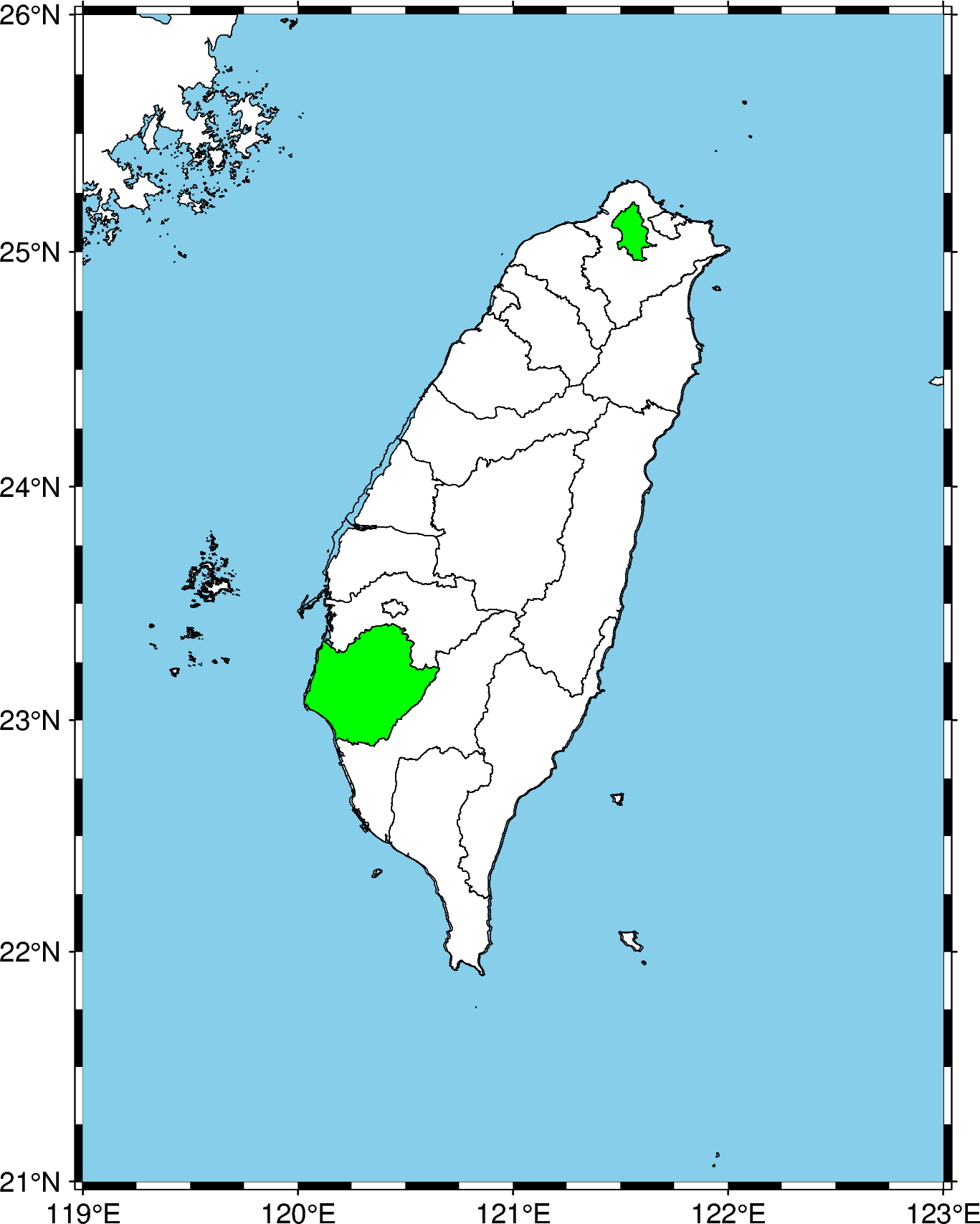
We selected the two counties to highlight on the map - Taipei City, Tainan City.

countiesShp = os.path.join("countiesData","COUNTY_MOI_1090820.shp")

gdf = gpd.read_file(countiesShp)

all_data = []
all_data.append(gdf[gdf["COUNTYENG"]=="Taipei City"])
all_data.append(gdf[gdf["COUNTYENG"]=="Tainan City"])

Plot basemap using PyGMT

Now, we can plot the simple basemap using PyGMT. The benefit of using PyGMT is that we don’t need the coastlines and topographic data separately and the output is high-resolution.

region = [119, 123, 21, 26]

fig = pygmt.Figure()
fig.basemap(region=region, projection="M4i", frame=True)

fig.coast( 
    water='skyblue', 
    shorelines=True)

Overlay the counties

Now, we can overlay the selected counties, fill them with green color, and then put all other counties with the background color (white).

for data_shp in all_data:
    fig.plot(data=data_shp,color="green")
fig.plot(data=countiesShp)

Save the map in raster and vector format

Now, we can save the map in raster and vector format for later use.

fig.savefig('map1.png')
fig.savefig('map1.pdf')

Topographic map

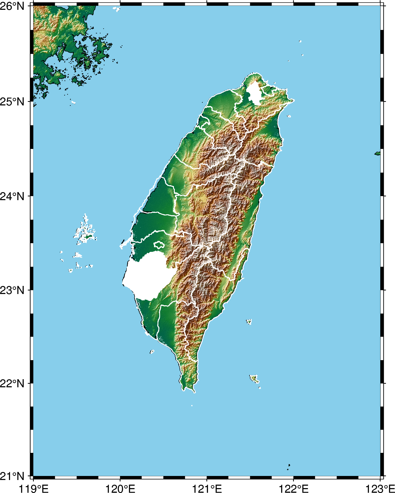
Instead of using simple white as background (which btw looks quite descent to me), we can use the topographic background:

import pygmt
import os
import geopandas as gpd

countiesShp = os.path.join("countiesData","COUNTY_MOI_1090820.shp")

gdf = gpd.read_file(countiesShp)

all_data = []
all_data.append(gdf[gdf["COUNTYENG"]=="Taipei City"])
all_data.append(gdf[gdf["COUNTYENG"]=="Tainan City"])


region = [119, 123, 21, 26]

fig = pygmt.Figure()
fig.basemap(region=region, projection="M4i", frame=True)
fig.grdimage("@srtm_relief_03s", shading=True, cmap='geo')

fig.coast( 
    water='skyblue', 
    shorelines=True)

for data_shp in all_data:
    fig.plot(data=data_shp,color="white", pen=["0.02c", 'white'])
fig.plot(data=countiesShp, pen=["0.02c", 'white'])

fig.savefig('map1.png')
fig.savefig('map1.pdf')

Plotting North America maps

Now, let us plot the map of NA using the combination of geopandas and PyGMT. You can obtain the shapefile data from the NOAA website.

Reading data

Here, we use the geopandas provided dataset. But the steps are similar for datasets from any other sources.

import os
import geopandas as gpd
import pygmt
import matplotlib.pyplot as plt

dataShp = os.path.join("GSHHS_shp","f","GSHHS_f_L1.shp")
# gdf = gpd.read_file(dataShp)
gdf = gpd.read_file(gpd.datasets.get_path('naturalearth_lowres'))

print(gdf.columns)
# print(gdf['source'].unique())
print(gdf.head())
# print(len(gdf))
print(gdf.crs) #“EPSG:4326” WGS84 Latitude/Longitude, used in GPS
# gdf = gdf.to_crs("EPSG:3395") #Spherical Mercator. Google Maps, OpenStreetMap, Bing Maps

Extract data for North America

Now, we use the Continents column of the geopandas dataframe to extract the data for North America.

na_gdf = gdf[gdf['continent'] == 'North America']

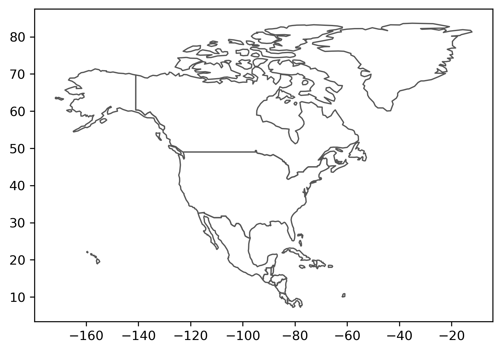
Plotting map using geopandas plot method

First we plot the map using the geopandas plot method.

fig, ax = plt.subplots(1, 1)
na_gdf.boundary.plot(ax=ax,  color="#555555", linewidth=1)
# na_gdf.plot(ax=ax,  color="#555555", linewidth=1)
plt.savefig('north-america-geopandas-map.png',bbox_inches='tight',dpi=300)
plt.close('all')

Plotting map using PyGMT

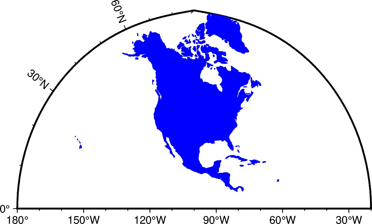
Now, we plot the map using the PyGMT.

# Define geographical range
minlon, maxlon = -180, -20
minlat, maxlat = 0, 90

fig = pygmt.Figure()
fig.basemap(region=[minlon, maxlon, minlat, maxlat], projection="Poly/4i", frame=True)
fig.plot(data=na_gdf,color="blue")
fig.savefig("north-america-pygmt-map.png", crop=True, dpi=300, transparent=True)

Conclusions

We have seen two cases (Taiwan and North America) of how to easily add the shapefile data on top of the PyGMT map. We plotted the counties data on top of the basemap of Taiwan. Furthermore, we created a high-resolution topographic map with shapefile data overlayed on it.

Recap

• Shapefile = geometry + attributes + index. .shp holds the shapes, .dbf the attribute table, .shx the spatial index — geopandas.read_file ties them together.
• Filter like a dataframe. A GeoDataFrame is a pandas DataFrame with a geometry column, so gdf[gdf["COUNTYENG"] == "Taipei City"] selects features by attribute.
• Hand it straight to PyGMT. fig.plot(data=gdf, fill=...) draws the selected geometry over your basemap (or a grdimage topographic background).
• Two modern gotchas: use fill= (not color=) in current PyGMT, and replace gpd.datasets.get_path('naturalearth_lowres') with a direct Natural Earth download on geopandas ≥ 1.0.

Where to go next

• PyGMT fig.plot docs (incl. fill): pygmt.org/latest/api/generated/pygmt.Figure.plot.html
• geopandas read_file: geopandas.org/en/stable/docs/reference/api/geopandas.read_file.html
• Natural Earth vector downloads: naturalearthdata.com/downloads