Time Series Analysis in Python: Filtering or Smoothing Data (codes included)

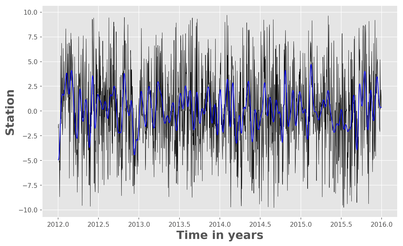
In this post, we will see how we can use Python to low-pass filter the 10 year long daily fluctuations of GPS time series. We need to use the “Scipy” package of Python.

The only important thing to keep in mind is the understanding of Nyquist frequency. The Nyquist or folding frequency half of the sampling rate of the discrete signal. To understand the concept of Nyquist frequency and aliasing, the reader is advised to visit this post. For filtering the time-series, we use the fraction of Nyquist frequency (cut-off frequency).

Code Description

Following are the codes and line by line explanation for performing the filtering in a few steps:

Import Libraries

• import numpy module for efficiently executing numerical operations
• import the pyplot from the matplotlib library
• predefine figure window size, and default figure settings
• use matplotlib ggplot style. I personally like to use “ggplot” style of graph for my work but it depends on the user’s preference whether they wanna use it.

import numpy as np
import matplotlib.pyplot as plt
from scipy import signal

from matplotlib import rcParams
rcParams['figure.figsize'] = (10.0, 6.0) #predefine the size of the figure window
rcParams.update({'font.size': 14}) # setting the default fontsize for the figure
rcParams['axes.labelweight'] = 'bold' #Bold font style for axes labels
from matplotlib import style
style.use('ggplot')

Load data

We load the data in the mat format (skipped) but this code will work for any sort of time series. If you have MiniSeed data, you can easily convert that to the MATLAB or mat format using the following utility:

# loading data part skipped (can be done using scipy for mat format data)
dN=np.array(data['dN'])
dE=np.array(data['dE'])
dU=np.array(data['dU'])
slat=np.array(data['slat'])[0]
slon=np.array(data['slon'])[0]
tdata=np.array(data['tdata'])[0]
stn_name=np.array(stn_info['stn_name'])[0]
stns=[stn_name[i][0] for i in range(len(stn_name))]

Visualizing the original and the Filtered Time Series

fig = plt.figure()
ax = fig.add_subplot(1, 1, 1)
indx=np.where( (tdata > 2012) & (tdata < 2016) )
ax.plot(tdata[indx],dU[indx,0][0],'k-',lw=0.5)

Filtering of the time series

fs=1/24/3600 #1 day in Hz (sampling frequency)

nyquist = fs / 2 # 0.5 times the sampling frequency
cutoff=0.1 # fraction of nyquist frequency, here  it is 5 days
print('cutoff= ',1/cutoff*nyquist*24*3600,' days') #cutoff=  4.999999999999999  days
b, a = signal.butter(5, cutoff, btype='lowpass') #low pass filter


dUfilt = signal.filtfilt(b, a, dU[:,0])
dUfilt=np.array(dUfilt)
dUfilt=dUfilt.transpose()

• Continue plotting on the exisitng figure window

ax.plot(tdata[indx],dUfilt[indx],'b',linewidth=1)

ax.set_xlabel('Time in years',fontsize=18)
ax.set_ylabel('Stations',fontsize=18)
plt.savefig('test.png',dpi=150,bbox_inches='tight')

Complete Script:

Output Figure:

Recap

• Filtering/smoothing separates a slow signal (trend) from fast noise — here, pulling a multi-year drift out of daily GPS fluctuations.
• A low-pass filter keeps frequencies below a cutoff; the cutoff is a fraction of the Nyquist frequency ($f_N = f_s/2$), the highest frequency a sampled series can represent.
• scipy.signal.butter(order, cutoff, btype='lowpass') designs a Butterworth filter; the cutoff is normalized to the Nyquist frequency (so 0.1 means 10 % of $f_N$).
• filtfilt applies the filter forward and backward for zero phase shift — the smoothed curve lines up in time with the original.
• Simpler time-domain smoothers — a moving average (np.convolve / pandas.rolling) or scipy.signal.savgol_filter — trade frequency precision for ease.

Where to go next

• Time series analysis in geophysics: loading and visualizing data — the previous tutorial: how to load the GPS series filtered here.
• Signal denoising using the Fast Fourier Transform — the Nyquist/aliasing background and a frequency-domain denoiser.
• Time-frequency analysis in MATLAB — when the frequency content changes over time.

This post was last modified at 2026-07-12 18:45.