How effective is the signal denoising using the MATLAB based wavelet analysis

Wavelets analysis can be thought of as a general form of Fourier Analysis. Fourier Transform is often used in denoising the signals. Still, the biggest downside of this approach is that the signal needs to be stationary. Most of our real-world measurements are not stationary. Also, in Fourier-based denoising, we apply a lowpass filter to remove the noise. However, when the data has high-frequency features such as spikes in a signal or edges in an image, the lowpass filter smooths these out.

Here, the wavelet-based approach might have some advantages. Wavelets look at the signals in the multi-resolution window. It localizes features in the signal to a different scale. We can take advantage of that and preserve important signals, and removing nonuniform noise. I have covered the basics of the multi-resolution analysis using wavelets in previous post.

Denoising using wavelets

When we take the wavelet transform of a time series, it concentrates the signal features in a few large-magnitude wavelet coefficients. In general, the coefficients that are smaller in value are considered noise. Theoretically, we can shrink those coefficients or simply remove them.

Obtain the real-world signal

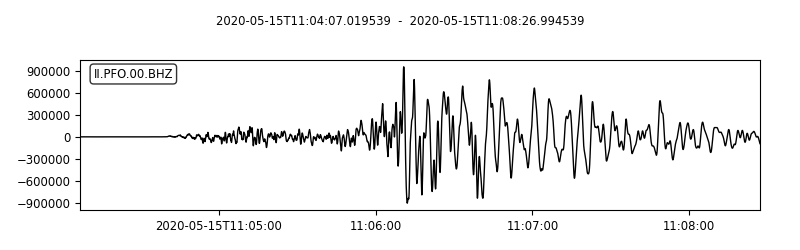
In this case, I will download the seismic time series recording a major earthquake. I will use the Obspy module to download the data from IRIS. For details on how to download waveforms using Obspy, see my previous post. I will download the waveforms for the arbitrarily selected event “2020-05-15 Mww 6.5 Nevada” located at (38.1689°N, 117.8497° W).

from obspy import read
from obspy.clients.fdsn import Client
from obspy import UTCDateTime
import matplotlib.pyplot as plt

client = Client("IRIS")

origin_time = UTCDateTime("2020-05-15T11:03:27Z")
net = "II"
stn = "PFO"
channel = "BHZ"
st = client.get_waveforms(net, stn, "00", channel,
                          origin_time+40, origin_time+300, attach_response=True)
st_copy = st.copy()
st_copy.remove_response(output="VEL")

# Filtering with a lowpass on a copy of the original Trace
st_copy[0].filter('highpass', freq=5.0, corners=2, zerophase=True)

st.plot(
    outfile="myStream.png",
)

print(st_copy)
st.write(f'{net}-{stn}-{channel}.mseed', format="MSEED")

1 Trace(s) in Stream:
II.PFO.00.BHZ | 2020-05-15T11:04:07.019539Z - 2020-05-15T11:08:26.994539Z | 40.0 Hz, 10400 samples

This saves the mseed data into the script directory as well the plot of the “stream”. I also highpass filtered the signal to obtain the high-frequency part of the time series.

Convert the mseed to mat format

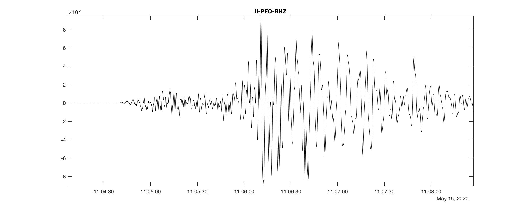
Now, we want to make the data MATLAB readable. I have written a utility to convert any mseed format data to mat format. I will use that in this case.

python convert_mseed_mat.py -inp II-PFO-BHZ.mseed

Denoise the signal using undecimated wavelet transform

I will use the Matlab function wdenoise to denoise the signal down to level 9 using the sym4 and db1 wavelets. wdenoise denoises the signal using an empirical Bayesian method with a Cauchy prior.

%% Using sym4
[XDEN,DENOISEDCFS] = wdenoise(data_double,9,'Wavelet','sym4','DenoisingMethod','BlockJS');
close;

fig2=figure('Renderer', 'painters', 'Position', [100 100 1000 400], 'color','w');
plot(data_double,'r')
hold on;
plot(XDEN, 'b')
legend('Original Signal','Denoised Signal')
axis tight;
hold off;
axis tight;
print(fig2,['denoise_signal_sym49','.jpg'],'-djpeg')

snrsym = -20*log10(norm(abs(data_double-XDEN))/norm(data_double))

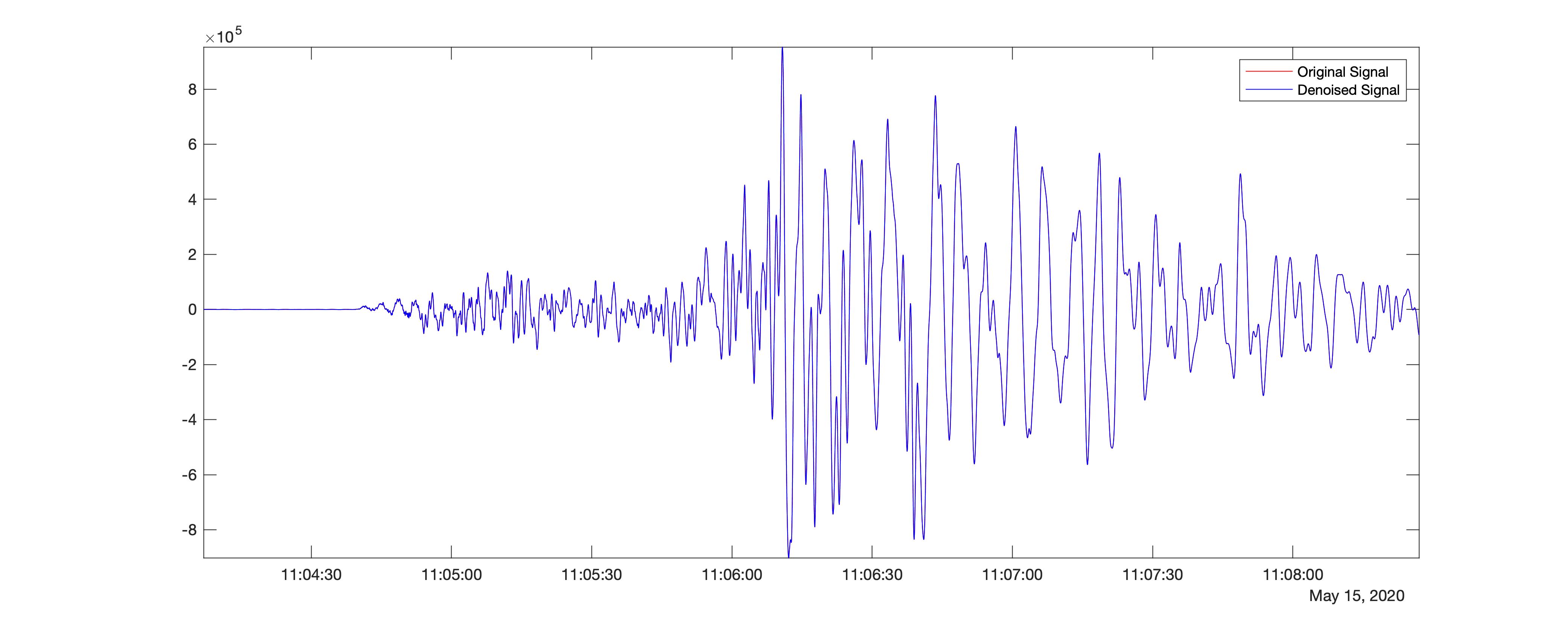
In the above code, I denoised the seismic time-series using level 9 using block thresholding by setting the name-value pair, ‘DenoisingMethod’,’BlockJS’. I used the wavelet sym4.

The resultant difference in the signal strength compared with the original time-series is 82.5786.

Further, I try the same procedure using a different wavelet - db1.

%% Using db1
[XDEN_db1,DENOISEDCFS2] = wdenoise(data_double,9,'Wavelet','db1','DenoisingMethod','BlockJS');
close;

fig3=figure('Renderer', 'painters', 'Position', [100 100 1000 400], 'color','w');
plot(data_double,'r')
hold on;
plot(XDEN_db1, 'b')
legend('Original Signal','Denoised Signal')
axis tight;
hold off;
axis tight;
print(fig3,['denoise_signal_db1','.jpg'],'-djpeg')

snrdb1 = -20*log10(norm(abs(data_double-XDEN_db1))/norm(data_double))

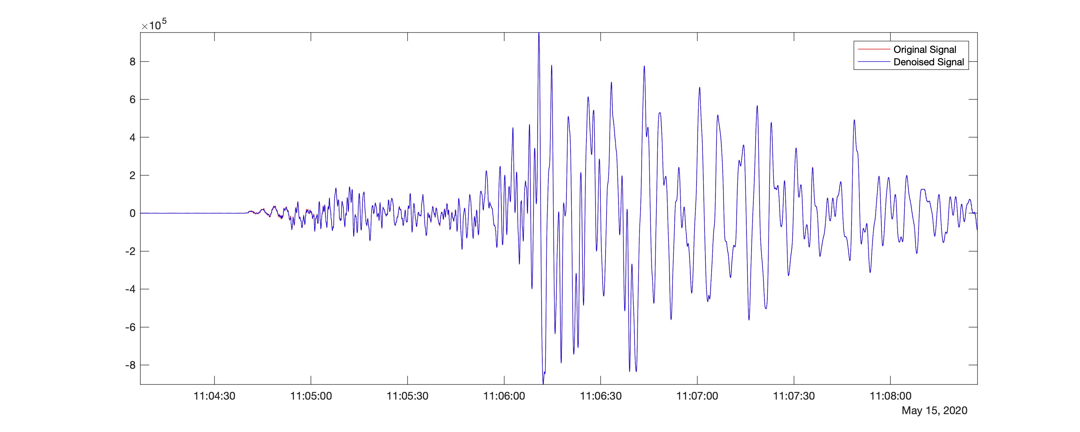
This gives the resultant difference in the signal strength compared with the original time-series to be 34.5294. Hence, we find that the difference is significant in the wavelet, sym4. We can also play with several other parameters, including the levels.

I tried to change the level to 2, 5, 10 and got the SNR to be 82.7493, 82.5789, 82.5786, respectively, for the “sym4” wavelet. The insignificant difference between the SNR for different levels may show that the amount of high-frequency noise is not excessive in this case. Let us try to verify this hypothesis using the noisy synthetic data (in this case, we will have complete control).

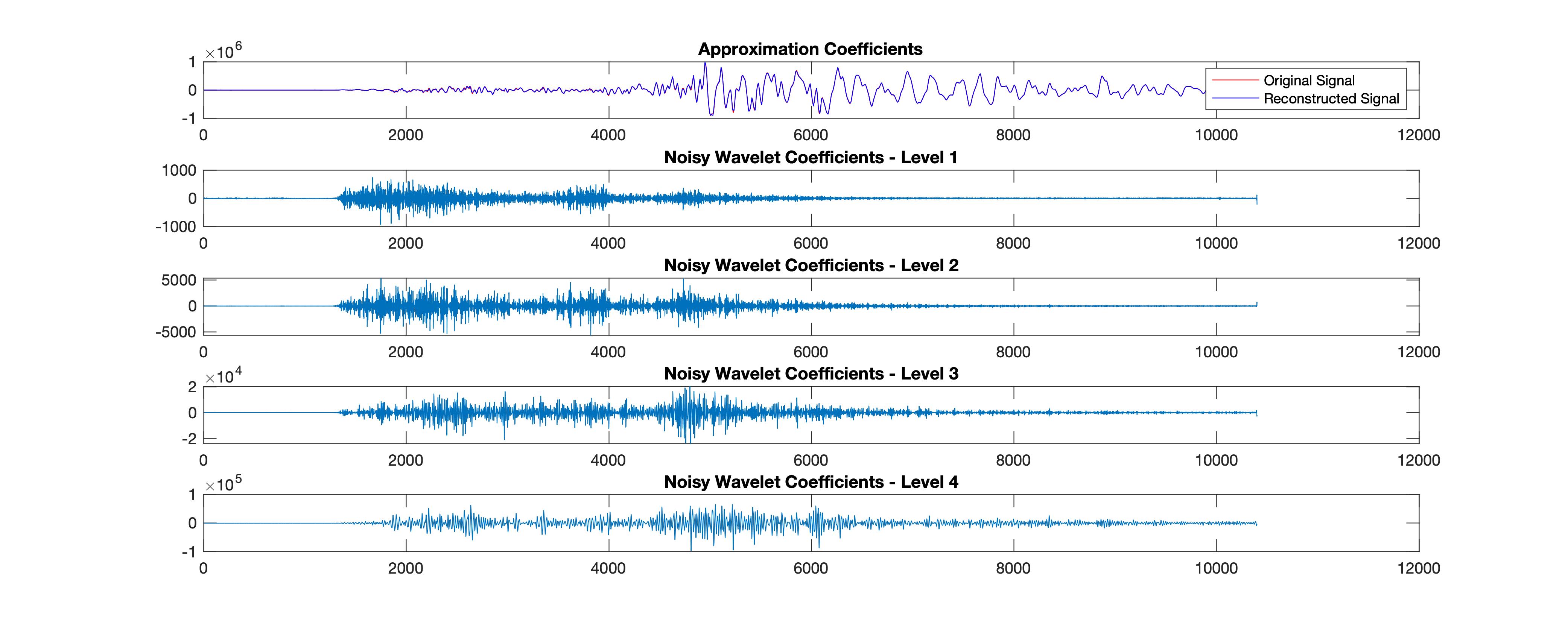
%% Plot reconstructions based on the level-4 approximation
[sigden,coefs] = cmddenoise(data_double,'sym4',4);
[C,L] = wavedec(data_double,4,'sym4');

fig5= figure('Renderer', 'painters', 'Position', [100 100 1000 400], 'color','w');
app = wrcoef('a',C,L,'sym4',4); %Coefficients to reconstruct, specified as 'a' or 'd', for approximation or detail coefficients, respectively.
subplot(5,1,1);
plot(data_double, 'r-')
title('Approximation Coefficients');
hold on;
plot(app, 'b'); 
legend('Original Signal','Reconstructed Signal')
for nn = 1:4
    det = wrcoef('d',C,L,'sym4',nn);
    subplot(5,1,nn+1)
    plot(det); title(['Noisy Wavelet Coefficients - Level '...
          num2str(nn)]);
end
print(fig5,['wavelet_reconstruction','.jpg'],'-djpeg')

Complete MATLAB code

clear; close; clc;
wdir='./';

fileloc0=[wdir,'II-PFO-BHZ'];
fileloc_ext = '.mat';
fileloc = [fileloc0 fileloc_ext];

if exist(fileloc,'file')
    disp(['File exists ', fileloc]);
    load(fileloc);
    
    all_stats = fieldnames(stats);
    all_data = fieldnames(data);
    
    for id=1
        %% read data and header information
        stats_0 = stats.(all_stats{id});
        data_0 = data.(all_data{id});
        
        sampling_rate = stats_0.('sampling_rate');
        delta = stats_0.('delta');
        starttime = stats_0.('starttime');
        endtime = stats_0.('endtime');
        t1 = datetime(starttime,'InputFormat',"yyyy-MM-dd'T'HH:mm:ss.SSS'Z'");
        t2 = datetime(endtime,'InputFormat',"yyyy-MM-dd'T'HH:mm:ss.SSS'Z'");
        datetime_array = t1:seconds(delta):t2;
        
        %% Plot waveforms
        fig = figure('Renderer', 'painters', 'Position', [100 100 1000 400], 'color','w');
        plot(t1:seconds(delta):t2, data_0, 'k-')
        title([stats_0.('network'),'-', stats_0.('station'), '-', stats_0.('channel')])
        axis tight;
        print(fig,[fileloc0, '_ts', num2str(id),'.jpg'],'-djpeg')
        data_double = double(data_0);
    
        %% Using sym4
        [XDEN,DENOISEDCFS] = wdenoise(data_double,9,'Wavelet','sym4','DenoisingMethod','BlockJS');
        close;
        
        fig2=figure('Renderer', 'painters', 'Position', [100 100 1000 400], 'color','w');
        plot(data_double,'r')
        hold on;
        plot(XDEN, 'b')
        legend('Original Signal','Denoised Signal')
        axis tight;
        hold off;
        axis tight;
        print(fig2,['denoise_signal_sym49','.jpg'],'-djpeg')
        
        snrsym = -20*log10(norm(abs(data_double-XDEN))/norm(data_double))
        
        %% Using db1
        [XDEN_db1,DENOISEDCFS2] = wdenoise(data_double,9,'Wavelet','db1','DenoisingMethod','BlockJS');
        close;
        
        fig3=figure('Renderer', 'painters', 'Position', [100 100 1000 400], 'color','w');
        plot(data_double,'r')
        hold on;
        plot(XDEN_db1, 'b')
        legend('Original Signal','Denoised Signal')
        axis tight;
        hold off;
        axis tight;
        print(fig3,['denoise_signal_db1','.jpg'],'-djpeg')
        
        snrdb1 = -20*log10(norm(abs(data_double-XDEN_db1))/norm(data_double))

    end
end

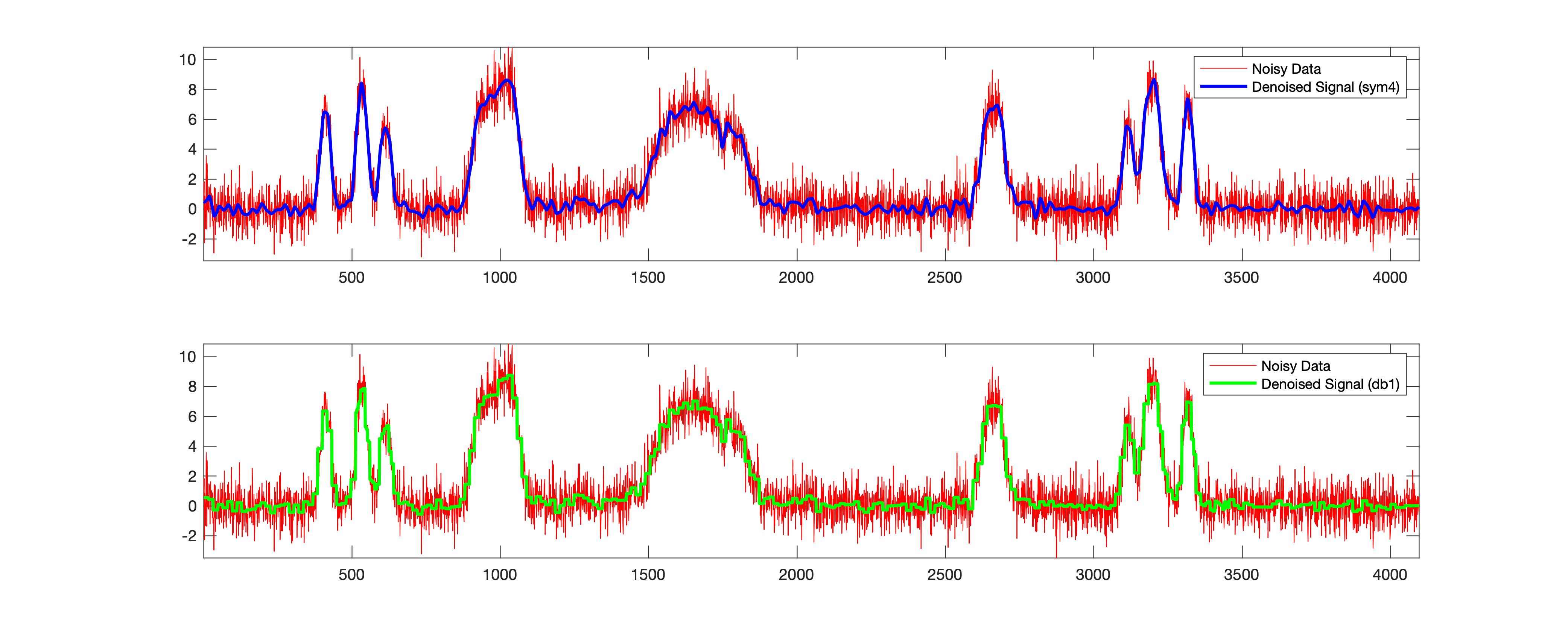
Wavelet denoising the noisy synthetic data

clear; close; clc;

rng default;
[X,XN] = wnoise('bumps',12,sqrt(6)); %returns values x of the test signal fun evaluated at 2n linearly spaced points from 0 to 1
denoised_signal = wdenoise(XN,4,'Wavelet','sym4','DenoisingMethod','BlockJS');
denoised_signal_db1 = wdenoise(XN,4,'Wavelet','db1','DenoisingMethod','BlockJS');


fig3=figure('Renderer', 'painters', 'Position', [100 100 1000 400], 'color','w');
ax1 = subplot(211)
plot(XN,'r')
hold on;
plot(denoised_signal,'b', 'linewidth',2)
legend('Noisy Data', 'Denoised Signal (sym4)')
hold off;
xlim([0, 4000])
axis tight;
ax2 = subplot(212)
plot(XN,'r')
hold on;
plot(denoised_signal_db1,'g', 'linewidth',2)
legend('Noisy Data', 'Denoised Signal (db1)')
hold off;
xlim([0, 4000])
axis tight;
linkaxes([ax1 ax2],'x')
print(fig3,['noisy_test_signal','.jpg'],'-djpeg')

snrsym = -20*log10(norm(abs(denoised_signal-XN))/norm(XN))
snrdb1 = -20*log10(norm(abs(denoised_signal_db1-XN))/norm(XN))

This example has been derived from the MATLAB example. In the above case, for the same data, I got the SNR to be 9.6994 and 9.4954 for sym4 and db1 wavelets. This also shows that there is a significant difference for the sym4. Please note that “sym4” works well in most cases and probably is the reason why it has been adopted as the default.

Conclusions

We have seen how to download seismic waveforms, convert them into mat format from mseed and then perform denoising using wavelet analysis. We first performed wavelet denoising on the high-frequency seismic time series, but after reconstruction, the difference is not apparent visually. But from the SNR, we can see the differences. We have also plotted the wavelet coefficients at different scales. Further, I have shown on a synthetic time-series how wavelet denoising works.

Recap

• Denoising = decompose → threshold → reconstruct. Transform to wavelet coefficients, shrink the small ones (noise), and invert.
• Why wavelets beat Fourier here. Localization in time and scale preserves spikes and edges that a lowpass filter would smear; wavelets also don’t require a stationary signal.
• Choice of wavelet matters. sym4 gave a larger SNR than db1 in both the real and synthetic tests — a reason sym4 is a common default.
• Level has limited effect here. Varying the decomposition level (2/5/10) barely changed the SNR, suggesting the high-frequency noise wasn’t excessive in this record.
• The API is current. wdenoise/cmddenoise/wavedec/wrcoef still ship in the Wavelet Toolbox; the interactive Wavelet Signal Denoiser app is a modern way to explore parameters.

Where to go next

• MATLAB wdenoise docs: mathworks.com/help/wavelet/ref/wdenoise.html
• Wavelet basics (previous post): Towards multi-resolution analysis with the wavelet transform
• The Fourier alternative: Signal denoising using the Fast Fourier Transform

References

1. Wu, W., & Cai, P. Simulation of Wavelet Denoising Based on MATLAB. Information and Electronic Engineering, 2008(03). CNKI abstract
2. MATLAB Wavelet Toolbox, The MathWorks, Inc. mathworks.com