A Quick Overview on Geospatial Data Visualization using PyGMT
PyGMT is a Python interface to the Generic Mapping Tools (GMT). This post is a quick tour: a topographic map, data points on it, earthquake focal mechanisms two ways, and a tomographic (velocity anomaly) map.
The one mental model
A PyGMT map is built up in layers, one method call at a time, each drawn on top of the last:
makecpt (colors) → grdimage (topography) → coast (shorelines) → plot/meca (your data) → colorbar (scale).
Order matters — later calls draw over earlier ones — and everything hangs off one fig = pygmt.Figure().
Install libraries
Using python env
python -m venv geoviz
source geoviz/bin/activate
pip install pygmt
- Try:
python -c "import pygmt"if there’s no
ImportError, then you are good to go.
NOTE:
If there’s any pygmt import problem, install GMT separately and link the libgmt.dylib file to the file python is looking for!
- One way to install GMT is
conda install gmt -c conda-forge
ln -s ~/miniconda3/envs/boxgmt/lib/libgmt.dylib ~/miniconda3/envs/geoviz/lib/libgmt.dylib
Using conda env (recommended)
conda create --name geoviz --channel conda-forge pandas pygmt jupyter notebook
Why conda is recommended: PyGMT wraps the GMT C library, so pip install pygmt only works if
GMT (≥ 6.5) is already installed — that’s the libgmt link dance in the note above. Installing from
conda-forge bundles GMT and PyGMT together and avoids all of it.
Import Libraries
import pygmt
import pandas as pd
import numpy as np
import xarray as xr
from scipy.interpolate import griddata
Plotting a topographic map
#define etopo data file
# topo_data = 'path_to_local_data_file'
topo_data = '@earth_relief_30s' #30 arc second global relief (SRTM15+V2.1 @ 1.0 km)
# topo_data = '@earth_relief_15s' #15 arc second global relief (SRTM15+V2.1)
# topo_data = '@earth_relief_03s' #3 arc second global relief (SRTM3S)

# define plot geographical range
minlon, maxlon = 60, 95
minlat, maxlat = 0, 25

# Visualization
fig = pygmt.Figure()

# make color pallets
pygmt.makecpt(
    cmap='topo',
    series='-8000/8000/1000',
    continuous=True
)

# plot high res topography
fig.grdimage(
    grid=topo_data,
    region=[minlon, maxlon, minlat, maxlat],
    projection='M4i',
    shading=True,
    frame=True
    )

# plot continents, shorelines, rivers, and borders
fig.coast(
    region=[minlon, maxlon, minlat, maxlat],
    projection='M4i',
    shorelines=True,
    frame=True
    )

# plot the topographic contour lines
fig.grdcontour(
    grid=topo_data,
    interval=4000,
    annotation="4000+f6p",
    limit="-8000/0", #to only display it below
    pen="a0.15p"
    )

# Plot colorbar
fig.colorbar(
    frame='+l"Topography"',
#     position="x11.5c/6.6c+w6c+jTC+v" #for vertical colorbar
    )

# save figure
save_fig = 0
if not save_fig:
    fig.show()
    #fig.show(method='external') #open with the default pdf reader
else:
    fig.savefig("topo-plot.png", crop=True, dpi=300, transparent=True)
#     fig.savefig("topo-plot.pdf", crop=True, dpi=720)
    print('Figure saved!')
Plotting data points on a topographic map
We plot 10 randomly generated coordinates on a topographic map with red circles. More symbol options can be found at the GMT site.
## Generate fake coordinates in the range for plotting
lons = minlon + np.random.rand(10)*(maxlon-minlon)
lats = minlat + np.random.rand(10)*(maxlat-minlat)

# define plot geographical range
minlon, maxlon = 60, 95
minlat, maxlat = 0, 25

# Visualization
fig = pygmt.Figure()

# make color pallets
pygmt.makecpt(
    cmap='topo',
    series='-8000/8000/1000',
    continuous=True
)

# plot high res topography
fig.grdimage(
    grid=topo_data,
    region=[minlon, maxlon, minlat, maxlat],
    projection='M4i',
    shading=True,
    frame=True
    )

# plot continents, shorelines, rivers, and borders
fig.coast(
    region=[minlon, maxlon, minlat, maxlat],
    projection='M4i',
    shorelines=True,
    frame=True
    )

# plot the topographic contour lines
fig.grdcontour(
    grid=topo_data,
    interval=4000,
    annotation="4000+f6p",
    limit="-8000/0", #to only display it only for the regions below the shorelines
    pen="a0.15p"
    )

# plot data points
fig.plot(
    x=lons,
    y=lats,
    style='c0.1i',
    color='red',
    pen='black',
    label='something',
    )

# save figure
fig.show()
#fig.show(method='external') #open with the default pdf reader
PyGMT version note: recent PyGMT (v0.12+) renamed the color parameter to fill in fig.plot
(and similar methods). The color='red' above still runs with a deprecation warning on current
versions; write fill='red' in new code.
Plotting focal mechanism on a map
Focal mechanisms in Harvard CMT convention
Using strike, dip, rake and magnitude
minlon, maxlon = 70, 100
minlat, maxlat = 0, 35

## Generate fake coordinates in the range for plotting
num_fm = 15
lons = minlon + np.random.rand(num_fm)*(maxlon-minlon)
lats = minlat + np.random.rand(num_fm)*(maxlat-minlat)

strikes = np.random.randint(low = 0, high = 360, size = num_fm)
dips = np.random.randint(low = 0, high = 90, size = num_fm)
rakes = np.random.randint(low = 0, high = 360, size = num_fm)
magnitudes = np.random.randint(low = 5, high = 9, size = num_fm)


fig = pygmt.Figure()

# make color pallets
pygmt.makecpt(
    cmap='topo',
    series='-8000/11000/1000',
    continuous=True
)

#plot high res topography
fig.grdimage(
    grid=topo_data,
    region='IN',
    projection='M4i',
    shading=True,
    frame=True
    )

fig.coast( region='IN',
    projection='M4i',
    frame=True,
    shorelines=True,
    borders=1, #political boundary
)

for lon, lat, st, dp, rk, mg in zip(lons, lats, strikes, dips, rakes, magnitudes):
    with pygmt.helpers.GMTTempFile() as temp_file:
        with open(temp_file.name, 'w') as f:
            f.write(f'{lon} {lat} 0 {st} {dp} {rk} {mg} 0 0') #moment tensor: lon, lat, depth, strike, dip, rake, magnitude
        with pygmt.clib.Session() as session:
            session.call_module('meca', f'{temp_file.name} -Sa0.2i')

fig.show()
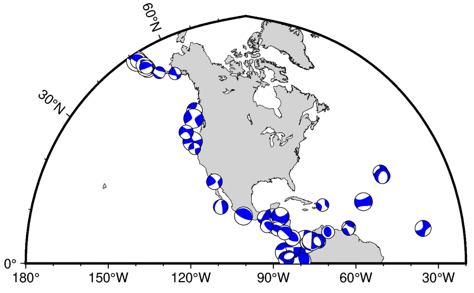
Focal mechanisms for Seismic moment tensor (Harvard CMT, with zero trace)
This example script needs formatted GCMT soln. Download the file from here
# Define geographical range
minlon, maxlon = -180, -20
minlat, maxlat = 0, 90


## Read GCMT sol
df_gcmt = pd.read_csv('gcmt_sol2.csv')

# ## Subset the data for the given geographical range (will make the program a bit faster to process)
# df_gcmt = df_gcmt[(df_gcmt['evlon'] >= minlon) & (df_gcmt['evlon'] <= maxlon) \
#                   & (df_gcmt['evlat'] >= minlat) & (df_gcmt['evlat'] <= maxlat)]
df_gcmt = df_gcmt[['evmag', 'evlat', 'evlon', 'evdep', 'm_rr','m_tt', 'm_pp', 'm_rt', 'm_rp', 'm_tp']]
df_gcmt.head()
fig = pygmt.Figure()


fig.basemap(region=[minlon, maxlon, minlat, maxlat], projection="Poly/4i", frame=True)

fig.coast(
        land="lightgrey",
        water="white",
        shorelines="0.1p",
        frame="WSNE",
        resolution='h',
        area_thresh=10000
    )

exponent = 16
factor = 10**exponent

#plotting moment tensor sols
for irow in range(len(df_gcmt)):
#     print(f"{irow}/{len(df_gcmt)-1}")
    m_rr = float(df_gcmt.loc[irow,'m_rr'])/factor
    m_tt = float(df_gcmt.loc[irow,'m_tt'])/factor
    m_pp = float(df_gcmt.loc[irow,'m_pp'])/factor
    m_rt = float(df_gcmt.loc[irow,'m_rt'])/factor
    m_rp = float(df_gcmt.loc[irow,'m_rp'])/factor
    m_tp = float(df_gcmt.loc[irow,'m_tp'])/factor
    evmag = float(df_gcmt.loc[irow,'evmag']) * 0.02
    evdep = float(df_gcmt.loc[irow,'evdep'])
    lat = float(df_gcmt.loc[irow,'evlat'])
    lon = float(df_gcmt.loc[irow,'evlon'])

    # store focal mechanisms parameters in a dict
    focal_mechanism = dict(mrr=m_rr, mtt=m_tt, mff=m_pp, mrt=m_rt, mrf=m_rp, mtf=m_tp, exponent=exponent)
    fig.meca(focal_mechanism, scale=f"{evmag}i", longitude=lon, latitude=lat, depth=evdep,G='blue')

fig.show()
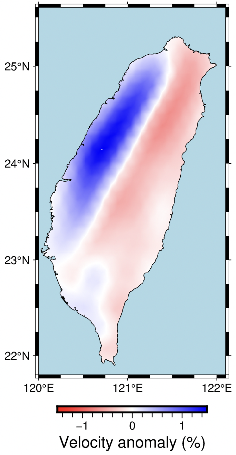
Tomographic data on a geographic map
datafile_dcg='dcg_080'

## Read perturbation data
df=pd.read_csv(datafile_dcg,delimiter='\s+', names=['longitude','latitude','pert', 'error'])
lons0=np.array(df['longitude'])
lats0=np.array(df['latitude'])
data=np.array(df['pert'])


coordinates0 = np.column_stack((lons0,lats0))
## Create structured data for plotting
minlon, maxlon = 120., 122.1
minlat, maxlat = 21.8, 25.6
step = 0.01

lons = np.arange(minlon, maxlon, step)
lats = np.arange(minlat, maxlat, step)

## interpolate data on spatial grid
xintrp, yintrp = np.meshgrid(lons, lats)
z1 = griddata(coordinates0, data, (xintrp, yintrp), method='cubic') #cubic interpolation
xintrp = np.array(xintrp, dtype=np.float32)
yintrp = np.array(yintrp, dtype=np.float32)

## xarray dataarray for plotting using pygmt
da = xr.DataArray(z1,dims=("lat", "long"),coords={"long": lons, "lat": lats},)
frame =  ["a1f0.25", "WSen"]

# Visualization
fig = pygmt.Figure()

# make color pallets
lim=abs(max(data.min(),data.max()))
# print(f'{data.min():.2f}/{data.max():.2f}')
pygmt.makecpt(
    cmap='red,white,blue',
    # series=f'{data.min()}/{data.max()}/0.01',
    series=f'-{lim}/{lim}/0.01',
    continuous=True
)

#plot high res topography
fig.grdimage(
    region=[minlon, maxlon, minlat, maxlat],
    grid=da,
    projection='M2i',
    interpolation='l'
    )

# plot coastlines
fig.coast(
    region=[minlon, maxlon, minlat, maxlat],
    shorelines=True,
    water="#add8e6",
    frame=frame,
    area_thresh=1000
    )


## Plot colorbar
# Default is horizontal colorbar
fig.colorbar(
    frame='+l"Velocity anomaly (%)"'
    )
fig.show()
Across all four examples, what stays the same?
Recap
Without scrolling up — what’s the PyGMT recipe? Every map here is the same layer stack:
makecptbuilds a colour palette,grdimagedraws the topography (or an interpolated data grid),coastadds shorelines/borders,- an overlay —
plot(points),meca(focal mechanisms), or the velocity grid — carries your data, colorbarlabels the scale.
Learn the stack once and every geospatial figure — earthquakes, focal mechanisms, tomography — is a variation on it.
Download notebook and resources
You can download the notebook and the resources from my github repo
Disclaimer of liability
The information provided by the Earth Inversion is made available for educational purposes only.
Whilst we endeavor to keep the information up-to-date and correct. Earth Inversion makes no representations or warranties of any kind, express or implied about the completeness, accuracy, reliability, suitability or availability with respect to the website or the information, products, services or related graphics content on the website for any purpose.
UNDER NO CIRCUMSTANCE SHALL WE HAVE ANY LIABILITY TO YOU FOR ANY LOSS OR DAMAGE OF ANY KIND INCURRED AS A RESULT OF THE USE OF THE SITE OR RELIANCE ON ANY INFORMATION PROVIDED ON THE SITE. ANY RELIANCE YOU PLACED ON SUCH MATERIAL IS THEREFORE STRICTLY AT YOUR OWN RISK.
Leave a comment