Topographic map clipped by coastlines in Python (codes included)
In this post, we demonstrate how to plot the clipped relief map in Python. For the previous post on “Plotting the geospatial data clipped by coastlines in Python”, see here. Here we use the same approach but instead of the geospatial dataset, we use the 1-arc minute topographic map we used in the previous plot.
We use the matplotlib’s Path module to deal with the polylines of the coastal path in Taiwan. The approach is simple (may not be so efficient computationally), we first plot the topography on the map, then select the polylines using the Path and then mask the region outside the coastline with lightblue color.
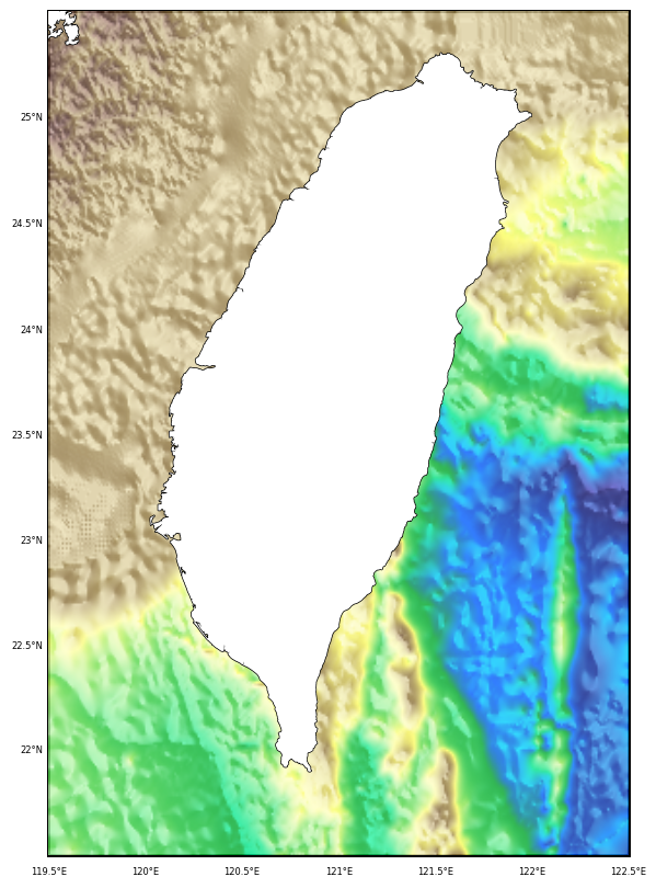
Key idea — draw everything, then mask the half you don’t want. Plot the full relief raster over the whole map, then build a matplotlib Path from the coastline polygons (map.landpolygons) and drop it on top as a high-zorder PathPatch. Change which polygons go into the patch and you flip what survives: include the map rectangle + coastlines and the patch fills the sea (leaving land topography); include only the coastlines and the patch fills the land in white (leaving the sea-floor bathymetry). Same trick, two opposite results.
Basemap is end-of-life (2026 update). mpl_toolkits.basemap had its final release in 2020 and is unmaintained — the maintained replacements are Cartopy and PyGMT. The code below still runs where Basemap is installed, and the clipping concept (build a PathPatch from coastlines, mask by zorder) transfers directly; in Cartopy you’d clip with set_boundary/a geometry mask, in PyGMT with a coastline clip.
Grid-file note. The code reads a hard-coded local file, ETOPO1_Bed_g_gmt4.grd — point this at your own downloaded ETOPO grid. ETOPO1 (2009) is still available, but NOAA NCEI’s current global relief model is now ETOPO 2022 (15 arc-second resolution, ~4× finer than ETOPO1), available in Ice-Surface and Bedrock versions.
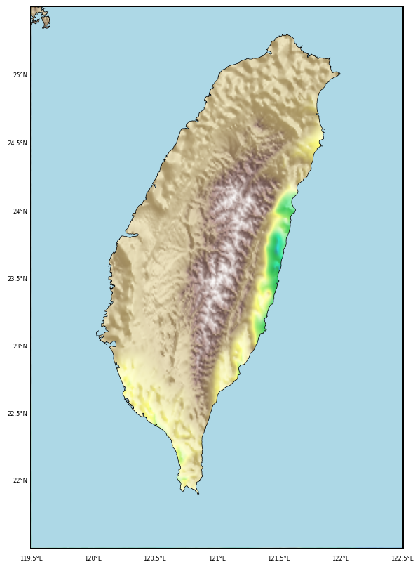
Basemap plot after clipping out the sea part
from mpl_toolkits.basemap import Basemap
import matplotlib.pyplot as plt
import numpy as np
import netCDF4 #you need to read gridded ETOPO1 file
import pandas as pd
from matplotlib.colors import LinearSegmentedColormap
from matplotlib.patches import Path, PathPatch
from matplotlib.colors import LightSource

etopo_file = "/Users/utpalkumar50/Documents/bin/ETOPO1_Bed_g_gmt4.grd"

lonmin, lonmax = 119.5,122.5
latmin, latmax = 21.5,25.5


fig, ax = plt.subplots(figsize=(10,10))
map = Basemap(projection='merc',resolution = 'f', area_thresh = 10000., llcrnrlon=lonmin, llcrnrlat=latmin,urcrnrlon=lonmax, urcrnrlat=latmax)
f = netCDF4.Dataset(etopo_file)
try:
    lons = f.variables['lon'][:]
    lats = f.variables['lat'][:]
    etopo = f.variables['z'][:]
except:
    lons = f.variables['x'][:]
    lats = f.variables['y'][:]
    etopo = f.variables['z'][:]


lonmin,lonmax = lonmin-1,lonmax+1
latmin,latmax = latmin-1,latmax+1

lons_col_index = np.where((lons>lonmin) & (lons<lonmax))[0]
lats_col_index = np.where((lats>latmin) & (lats<latmax))[0]

etopo_sl = etopo[lats_col_index[0]:lats_col_index[-1]+1,lons_col_index[0]:lons_col_index[-1]+1]
lons_sl = lons[lons_col_index[0]:lons_col_index[-1]+1]
lats_sl = lats[lats_col_index[0]:lats_col_index[-1]+1]
lons_sl, lats_sl = np.meshgrid(lons_sl,lats_sl)

ls = LightSource(azdeg=315, altdeg=45)
rgb = ls.shade(np.array(etopo_sl), cmap=plt.cm.terrain, vert_exag=1, blend_mode=ls.blend_soft_light)

map.imshow(rgb,zorder=2,alpha=0.8,cmap=plt.cm.terrain, interpolation='bilinear')

# Use a proxy artist for the colorbar...
cs = map.imshow(np.array(etopo_sl), cmap=plt.cm.terrain)
cs.remove()
fig.colorbar(cs, ax=ax, shrink=0.8)

map.drawcoastlines(color='k',linewidth=1,zorder=3)
map.drawcountries(color='k',linewidth=1,zorder=3)

parallelmin,parallelmax = int(latmin), int(latmax)+1
map.drawparallels(np.arange(parallelmin, parallelmax+1,0.5).tolist(),labels=[1,0,0,0],linewidth=0,fontsize=6)
meridianmin,meridianmax = int(lonmin),int(lonmax)+1
map.drawmeridians(np.arange(meridianmin, meridianmax+1,0.5).tolist(),labels=[0,0,0,1],linewidth=0,fontsize=6)
map.drawmapboundary(color='k', linewidth=2, zorder=1)


## Masking the topography outside Taiwan coastlines
x0,x1 = ax.get_xlim()
y0,y1 = ax.get_ylim()
map_edges = np.array([[x0,y0],[x1,y0],[x1,y1],[x0,y1]])
##getting all polygons used to draw the coastlines of the map
polys = [p.boundary for p in map.landpolygons]
##combining with map edges
polys = [map_edges]+polys[:]
##creating a PathPatch
codes = [[Path.MOVETO]+[Path.LINETO for p in p[1:]] for p in polys]
verts = [v for p in polys for v in p]
codes = [xx for cs in codes for xx in cs]

path = Path(verts, codes)
patch = PathPatch(path,facecolor='lightblue', edgecolor='none',zorder=4)

##masking the data outside the inland of taiwan
ax.add_patch(patch)

plt.savefig('station_map_masked.png',bbox_inches='tight',dpi=300)
plt.close('all')
Basemap plot after clipping out the land part
It is also possible to reverse the masking and keep the bathymetry of the region and mask the land region with white.
from mpl_toolkits.basemap import Basemap
import matplotlib.pyplot as plt
import numpy as np
import netCDF4
import pandas as pd
from matplotlib.colors import LinearSegmentedColormap
from matplotlib.patches import Path, PathPatch
from matplotlib.colors import LightSource


etopo_file = "/Users/utpalkumar50/Documents/bin/ETOPO1_Bed_g_gmt4.grd"

lonmin, lonmax = 119.5,122.5
latmin, latmax = 21.5,25.5


fig, ax = plt.subplots(figsize=(10,10))
map = Basemap(projection='merc',resolution = 'f', area_thresh = 10000., llcrnrlon=lonmin, llcrnrlat=latmin,urcrnrlon=lonmax, urcrnrlat=latmax)
f = netCDF4.Dataset(etopo_file)
try:
    lons = f.variables['lon'][:]
    lats = f.variables['lat'][:]
    etopo = f.variables['z'][:]
except:
    lons = f.variables['x'][:]
    lats = f.variables['y'][:]
    etopo = f.variables['z'][:]


lonmin,lonmax = lonmin-1,lonmax+1
latmin,latmax = latmin-1,latmax+1

lons_col_index = np.where((lons>lonmin) & (lons<lonmax))[0]
lats_col_index = np.where((lats>latmin) & (lats<latmax))[0]

etopo_sl = etopo[lats_col_index[0]:lats_col_index[-1]+1,lons_col_index[0]:lons_col_index[-1]+1]
lons_sl = lons[lons_col_index[0]:lons_col_index[-1]+1]
lats_sl = lats[lats_col_index[0]:lats_col_index[-1]+1]
lons_sl, lats_sl = np.meshgrid(lons_sl,lats_sl)

ls = LightSource(azdeg=315, altdeg=45)
rgb = ls.shade(np.array(etopo_sl), cmap=plt.cm.terrain, vert_exag=1, blend_mode=ls.blend_soft_light)

map.imshow(rgb,zorder=2,alpha=0.8,cmap=plt.cm.terrain, interpolation='bilinear')


map.drawcoastlines(color='k',linewidth=1,zorder=3)
map.drawcountries(color='k',linewidth=1,zorder=3)

parallelmin,parallelmax = int(latmin), int(latmax)+1
map.drawparallels(np.arange(parallelmin, parallelmax+1,0.5).tolist(),labels=[1,0,0,0],linewidth=0,fontsize=6)
meridianmin,meridianmax = int(lonmin),int(lonmax)+1
map.drawmeridians(np.arange(meridianmin, meridianmax+1,0.5).tolist(),labels=[0,0,0,1],linewidth=0,fontsize=6)
map.drawmapboundary(color='k', linewidth=2, zorder=1)


##getting all polygons used to draw the coastlines of the map
polys = [p.boundary for p in map.landpolygons]
##combining with map edges
polys = polys[:]
##creating a PathPatch
codes = [[Path.MOVETO]+[Path.LINETO for p in p[1:]] for p in polys]
verts = [v for p in polys for v in p]
codes = [xx for cs in codes for xx in cs]

path = Path(verts, codes)
patch = PathPatch(path,facecolor='white', edgecolor='none',zorder=4)

##masking the data outside the inland of taiwan
ax.add_patch(patch)


plt.savefig('station_map_masked_reverse.png',bbox_inches='tight',dpi=300)
plt.close('all')
Quick check: Why is the masking PathPatch added with a high zorder (here zorder=4)?
- Because
zordersets the colour of the coastline - So the mask is drawn on top of the relief raster (lower zorder), hiding the side you want to clip
- Because Basemap requires zorder to project coordinates
- It controls the resolution of the ETOPO grid
Recap
- To clip a relief map by coastlines: draw the full topography, then cover part of it with a
PathPatchbuilt from the coastline polygons at a highzorder. - Keep land → build the patch from map edges +
map.landpolygonsso it fills the sea; keep sea → build it from the land polygons only so it fills the land white. - The relief raster is a hill-shaded ETOPO grid read with
netCDF4and shaded via matplotlib’sLightSource. - The same clipping recipe works for any gridded field, not just topography.
- Basemap is EOL — the concept ports to Cartopy/PyGMT for new work.
Where to go next
- Plotting geospatial data clipped by coastlines — the same mask applied to a data field instead of topography.
- Shaded topographic map in Python — the hill-shaded ETOPO base this post clips.
- High-resolution topographic maps with PyGMT — the maintained, modern way to make relief maps.
Download codes here.
Disclaimer of liability
The information provided by the Earth Inversion is made available for educational purposes only.
Whilst we endeavor to keep the information up-to-date and correct. Earth Inversion makes no representations or warranties of any kind, express or implied about the completeness, accuracy, reliability, suitability or availability with respect to the website or the information, products, services or related graphics content on the website for any purpose.
UNDER NO CIRCUMSTANCE SHALL WE HAVE ANY LIABILITY TO YOU FOR ANY LOSS OR DAMAGE OF ANY KIND INCURRED AS A RESULT OF THE USE OF THE SITE OR RELIANCE ON ANY INFORMATION PROVIDED ON THE SITE. ANY RELIANCE YOU PLACED ON SUCH MATERIAL IS THEREFORE STRICTLY AT YOUR OWN RISK.
Leave a comment