Easy Statistical Analysis using the tools of MATLAB (codes included)
Loading likes…
“Technological innovations such as reconnaissance satellites are capable of spewing out data in volumes that defy conventional methods of interpretation. In the words of John Griffiths, “we must be able to digest the mass before it becomes a mess.” Only computer implemented mathematical and statistical tech- niques are powerful enough and fast enough to perform the task.” - J.C. Davis

Key idea — describe the data, then test a claim about it. Descriptive statistics compress a dataset into a few numbers that capture its centre (mean, median), its spread (standard deviation, interquartile range), and its shape (skewness = asymmetry, kurtosis = tail-heaviness). Inferential statistics then ask whether a pattern is real: the one-sample t-test measures how far the sample mean sits from a hypothesized value, scaled by the scatter — a large $|t|$ (small $p$) means the difference is unlikely to be chance. MATLAB gives you both in a few built-ins: mean, std, median, prctile, skewness, kurtosis, and ttest/ttest2.
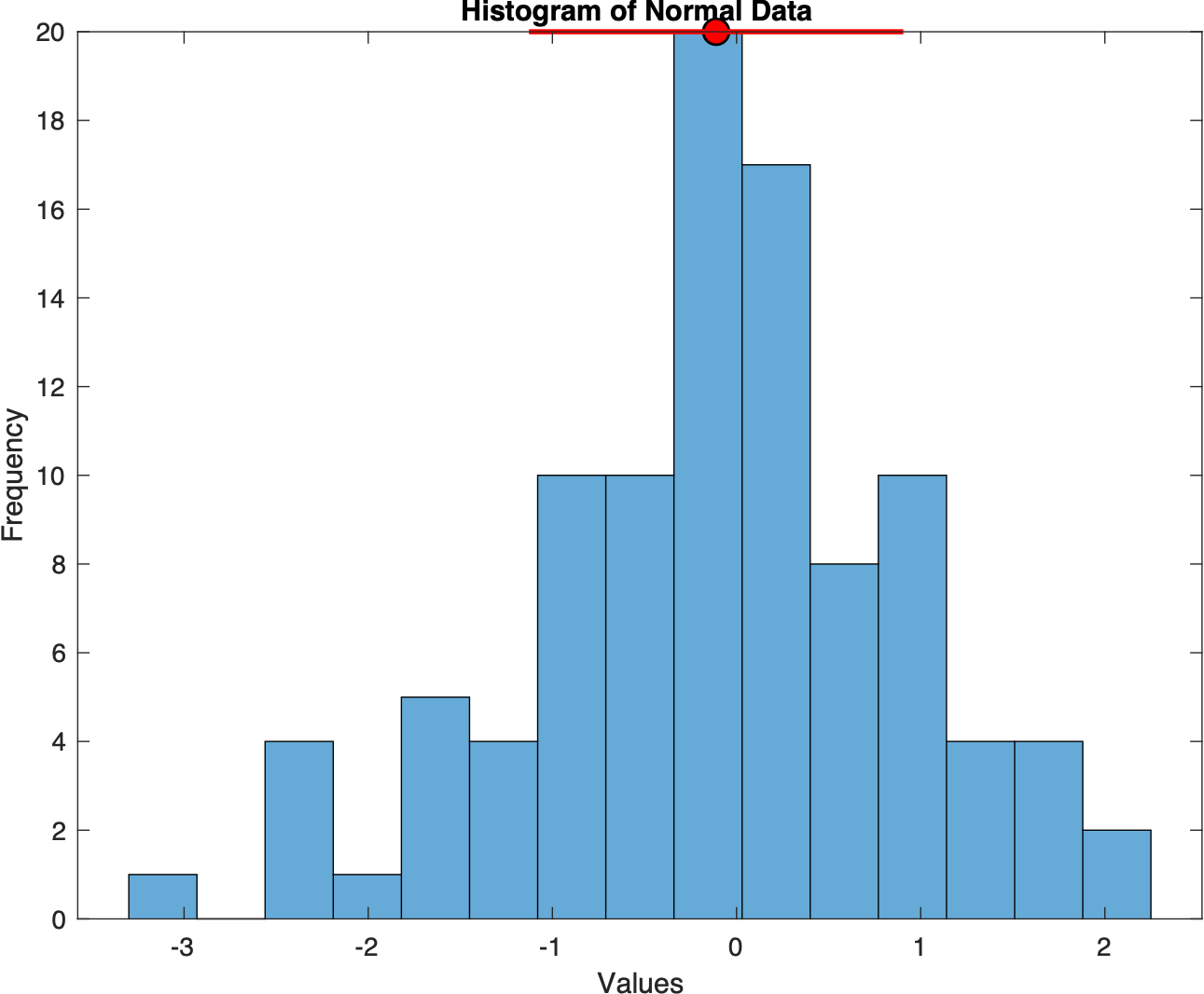
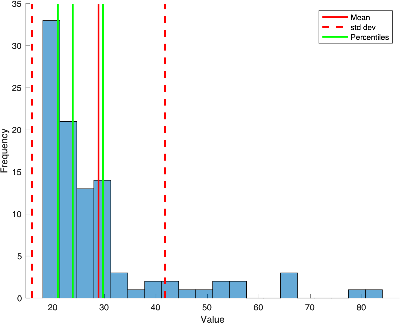
Analyzing random (normal and non-normal) data to perform basic statistical analysis
- Generate histograms
- plot mean and standard deviation
- compute and plot percentiles
%% Analysing random data to learn statistical skills
clear; close all; clc;

%% Normal Data
figure(1)
dataNormal=randn(100,1);
h1=histogram(dataNormal,15);
xlabel('Values'), ylabel('Frequency')
title('Histogram of Normal Data')
hold on
mu=mean(dataNormal);
sd=std(dataNormal);
binmax = max(h1.Values); %finding the maximum bin height
plot(mu,binmax,'ko','markerfacecolor','r', 'markersize',10); %plotting the location of mean
plot([mu-sd, mu+sd],[binmax, binmax], '-r', 'linewidth', 2); %plotting the 1 std
saveas(gcf,"normal_data_stats",'pdf')


%% Non-Normal Data
% generate some fake data
x = (randn(1,100).^2)*10 + 20;

% compute some simple data summary metrics
mn = mean(x);  % compute mean
sd = std(x);   % compute standard deviation
ptiles = prctile(x,[25 50 75]);  % compute percentiles (median and central 68%)

% make a figure
figure;
hold on;
histogram(x,20);  % plot a histogram using twenty bins
ax = axis;   % get the current axis bounds
  % plot lines showing mean and +/- 1 std dev
h1 = plot([mn mn],      ax(3:4),'r-','LineWidth',2);
h2 = plot([mn-sd mn-sd],ax(3:4),'r--','LineWidth',2);
h3 = plot([mn+sd mn+sd],ax(3:4),'r--','LineWidth',2);
  % plot lines showing percentiles
h4 = [];
for p=1:length(ptiles)
  h4(p) = plot(repmat(ptiles(p),[1 2]),ax(3:4),'g-','LineWidth',2);
end
legend([h1 h2 h4(1)],{'Mean' 'std dev' 'Percentiles'});
xlabel('Value');
ylabel('Frequency');
saveas(gcf,"non_normal_data_stats",'pdf')
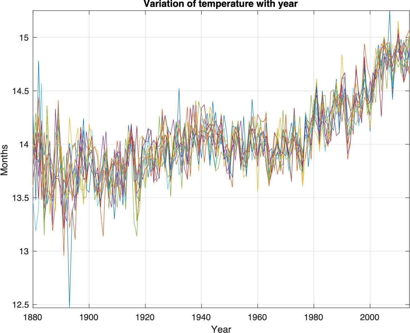
Global monthly temperature data
- Plot temperature data vs year
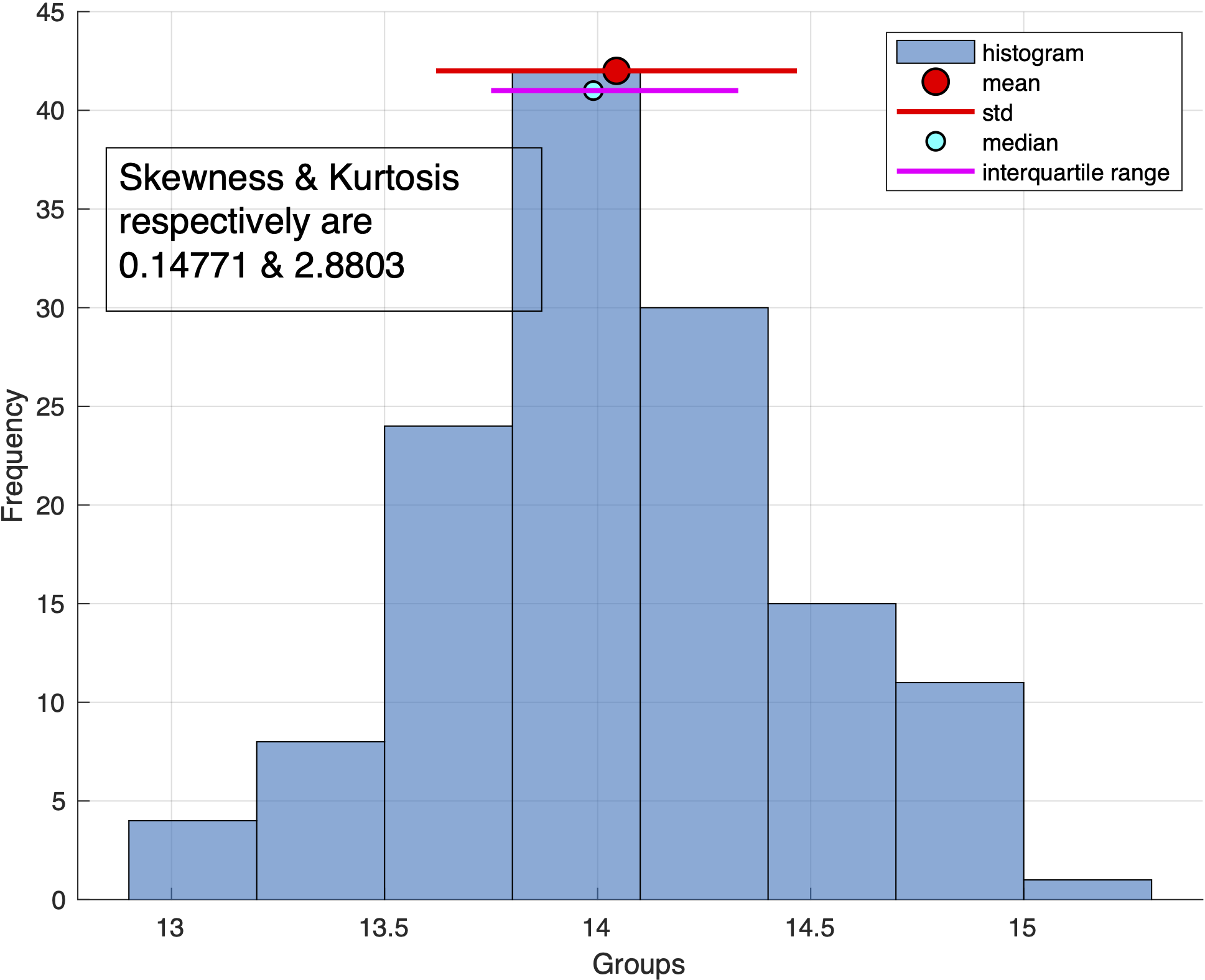
- compute basic statistics: mean, median, std, interquartile range, skewness, kurtosis
- plot histogram and statistics on it
clear; close all; clc;
load temp_month

%% Making a matrix of data
p=[Jan,Feb,Mar,Apr,May,Jun,Jul,Aug,Sep,Oct,Nov,Dec];
pstring={'Jan','Feb','Mar','Apr','May','Jun','Jul','Aug','Sep','Oct','Nov','Dec'};

[row, col]=size(p);
%% Plotting the data vs year
figure
for i=1:col
  plot(Year,p(:,i))
  grid on
  hold on
end
title('Variation of Months with Year')
xlabel('Year'), ylabel('Months')
axis tight
saveas(gcf,"dataYear",'pdf')

%% Statistical Analysis
for i=1:col
    dd=p(:,i);
    mu(i)=mean(dd); %mean
    sd(i)=std(dd); %standard deviation
    med(i)=median(dd); %median
    x = min(dd):0.01:max(dd);
    ddsorted = sort(dd,'ascend'); %interquartile range
    e25=ceil(25/100*length(dd)); e75=ceil(75/100*length(dd));
    iqr_dd = ddsorted([e25, e75]);
    skew_dd=skewness(dd);
    kurt_dd = kurtosis(dd);


    %Plotting Figure
    figure
  %  subplot(2,2,[1 2])
     xlabel('Groups'), ylabel('Frequency'),grid on
    annotation('textbox',...
    [0.15 0.65 0.3 0.15],...
    'String',{'Skewness & Kurtosis respectively are ',[num2str(skew_dd),' & ', num2str(kurt_dd)]},...
    'FontSize',14,...
    'FontName','Arial')
    hold on
    h1=histogram(dd,'BinMethod','auto');
    binmax1(i) = max(h1.Values); %finding the maximum bin height
    plot(mu(i),binmax1(i),'ko','markerfacecolor','r', 'markersize',10); %plotting the location of mean
    plot([mu(i)-sd(i), mu(i)+sd(i)],[binmax1(i), binmax1(i)], '-r', 'linewidth', 2); %plotting the 1 std
    plot(med(i),binmax1(i)-1,'ko','markerfacecolor','c', 'markersize',7)
    plot(iqr_dd,[binmax1(i)-1, binmax1(i)-1], '-m', 'linewidth',2);
    legend('histogram','mean','std','median','interquartile range')
    saveas(gcf,sprintf("hist_Month%s",pstring{i}),'pdf')
end
T-statistic
The uncertainty in the estimation of the population statistics can be accounted for by using a probability distribution that has a wider “spread” than the normal distribution. One such probability distribution is called the t distribution (similar to the normal distribution). It is dependent upon the size of the sample taken. When the number of observations in the sample is infinite, the t distribution and the normal distribution are identical.
The t-statistic is the ratio of the departure of the estimated value of a parameter from its hypothesized value to its standard error. t-tests are useful for establishing the likelihood that a given sample could be a member of a population with specified characteristics, or for testing hypotheses about the equivalency of two samples.
For a dataset with samples randomly collected from a normal population, the t-statistic may be computed by
\[t = \frac{\bar{X}-\mu_0}{s/\sqrt{n}}\]where,
$\bar{X}$: mean of the sample
$\mu_0$: hypothetical mean of population
$n$: number of obervations
$s$: standard deviation of observations
The numerator $\bar{X}-\mu_0$ is how far the sample mean is from the value you are testing. The denominator $s/\sqrt{n}$ is the standard error — the typical scatter of the sample mean, which shrinks as the sample grows. So $t$ is a signal-to-noise ratio: a difference of a given size counts for more when the data are tight (small $s$) or plentiful (large $n$). You compare the computed $t$ against a critical value from the Student’s-$t$ table at $n-1$ degrees of freedom and your chosen significance level $\alpha$.
Example
Let us taken the example from Davis (1986) for the porosity measurements.
| Sample number | Porosity (%) |
|---|---|
| 01 | 13 |
| 02 | 17 |
| 03 | 15 |
| 04 | 23 |
| 05 | 27 |
| 06 | 29 |
| 07 | 18 |
| 08 | 27 |
| 09 | 20 |
| 10 | 24 |
We wish to test that about samples came from the population having porosity of more than 18%.
Hypothesis test
Here, our null hypothesis is:
\[H_0: \mu_1 \leq \mu_0\]Alternative hypothesis:
\[H_1: \mu_1 \geq \mu_0\]In this test, we assume the mean, $\mu_0$, $s$ is estimated. For the above dataset of 10 samples, the degrees of freedom is 9.
We reject the null hypothesis only if the mean porosity significantly exceeds 18%. If we wish to test this hypothesis with the probability of rejecting it when it is true only one is twenty times ($\alpha = 0.05$), the computed value of t must exceed 1.833 for a one-tailed test. See here for the table of the Stduent’s t distribution with $\nu$ degrees of freedom.
The obtained value of 1.89 exceeds the critical value of t for nine degrees of freedom and 5% level of significance and hence lies in the critical region or region of rejection. Hence, we can reject the null hypothesis, leaving us with the alternative hypothesis that the porosity of the population from which the dataset was sampled is greater than 18%. Note that if the null hypothesis were accepted, we could only say that there is nothing in the sample to suggest that the population means is greater than 18%.
Computing t-statistic using MATLAB
clear; close all; clc;
% generate some fake data
data1=randn(100,1);
data2=(randn(150,1).^2)*10 + 20;
mu_x=mean(data1)
mu_y=mean(data2)
%t-statistic
[h,p,ci,stats] = ttest2(data1,data2,0.05,'both','unequal')
mu_x = -0.0727

mu_y = 29.8633

h = 1

p = 7.6969e-54

ci =
  -32.3794
  -27.4925

stats =
  struct with fields:
    tstat: -24.2062
       df: 150.9778
       sd: [2×1 double]
Quick check: In the porosity example the computed $t = 1.89$ exceeds the critical value $1.833$ at $\alpha = 0.05$ with 9 degrees of freedom. What does that let you conclude?
- The sample mean equals the hypothesized 18% exactly
- The result falls in the rejection region, so you reject $H_0$ — the population mean porosity is significantly greater than 18%
- Nothing, because $t$ must be negative to be significant
- The data must be re-collected because $t > 1$
Recap
- Descriptive statistics summarise centre (
mean,median), spread (std, interquartile range viaprctile), and shape (skewness,kurtosis) — visualise them on a histogram. - Symmetric data have mean ≈ median and skewness ≈ 0; skewed data pull the mean toward the long tail.
- The one-sample t-test compares a sample mean to a hypothesized value: $t = (\bar{X}-\mu_0)/(s/\sqrt{n})$, judged at $n-1$ degrees of freedom.
- Reject $H_0$ when $t$ lands in the critical region (here $t=1.89 > 1.833$) — or, in code, when MATLAB’s
ttest/ttest2returnsh = 1with a smallp. - MATLAB’s
ttest2also reports the confidence interval and astatsstruct withtstat,df, andsd.
Where to go next
- Hypothesis testing — null vs. alternative hypotheses, p-values and error types in depth.
- Monte Carlo simulations and correlations — a computational, resampling take on the same statistical questions.
References:
Davis, J. C. (1986). Statistics and data analysis in geology (2nd ed.). Wiley. https://search.worldcat.org/title/Statistics-and-data-analysis-in-geology/oclc/1422027856
Resources
- Kay, K. Lectures on Statistics and Data Analysis in MATLAB (archived).
- Wikipedia: t-statistic
Found this article useful?
Loading likes…
Disclaimer of liability
The information provided by the Earth Inversion is made available for educational purposes only.
Whilst we endeavor to keep the information up-to-date and correct. Earth Inversion makes no representations or warranties of any kind, express or implied about the completeness, accuracy, reliability, suitability or availability with respect to the website or the information, products, services or related graphics content on the website for any purpose.
UNDER NO CIRCUMSTANCE SHALL WE HAVE ANY LIABILITY TO YOU FOR ANY LOSS OR DAMAGE OF ANY KIND INCURRED AS A RESULT OF THE USE OF THE SITE OR RELIANCE ON ANY INFORMATION PROVIDED ON THE SITE. ANY RELIANCE YOU PLACED ON SUCH MATERIAL IS THEREFORE STRICTLY AT YOUR OWN RISK.
Leave a comment