Monte Carlo Simulation to test for the correlation between two dataset in MATLAB (codes included)
Loading likes…
Monte Carlo Simulations (MCS) can be used to extract important informations from the dataset that would be impossible to assess otherwise. Using MCS rather than the traditional methods to find the relation between two datasets are more intuitive.
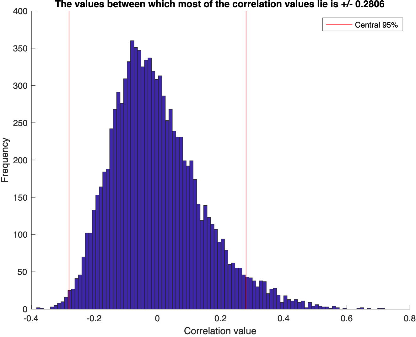
Key idea — build the “by chance” distribution, then see if your correlation beats it. Instead of trusting a formula, Monte Carlo simulates the null hypothesis directly: draw two independent random samples (which have no true relationship), compute their correlation, and repeat thousands of times. The result is a null distribution — the spread of correlation values you’d expect from pure chance. If a correlation you measured in real data falls outside the central 95 % of that distribution, it’s unlikely to be an accident, so you call it significant. It’s the same logic as a permutation test: let the computer show you what randomness looks like.
What is Monte Carlo Simulations??
MCS studies are computer-driven experimental investigations in which certain parameters, such as population means and standard deviations that are known a priori, are used to generate random (but plausible) sample data (Mooney 1997). These generated data are then used to evaluate the sampling behavior of one or more statistics of interest. This process of generating and analyzing data is repeated over many iterations and differing conditions that are thought to influence the sampling behavior of the statistic of interest (e.g., through increasing sample size, mean differences, variability). (Sigal & Chalmers, 2016, p. 137)
%%Monte Carlo simulations of correlation values
clear; close all; clc;
% define
numsim = 10000;   % number of simulations to run
samplesize = 50;  % number of data points in each sample

% pre-allocate the results vector
results = zeros(1,numsim);

% loop over simulations
for num=1:numsim

  % draw two sets of random numbers, each from the normal distribution
  data = (randn(samplesize,2).^2)*10+20;

  % compute the correlation between the two sets of numbers and store the result
  results(num) = corr(data(:,1),data(:,2));

end
% visualize the results
figure; hold on;
hist(results,100);
% ax = axis;
% mx = max(abs(ax(1:2)));  % make the x-axis symmetric around 0
% axis([-mx mx ax(3:4)]);
xlabel('Correlation value');
ylabel('Frequency');
%%
val = prctile(abs(results),95);
val
%%

% visualize this on the figure
ax = axis;
h1 = plot([val val],ax(3:4),'r-');
h2 = plot(-[val val],ax(3:4),'r-');
legend(h1,'Central 95%');
title(sprintf('The values between which most of the correlation values lie is +/- %.4f',val));
saveas(gcf,"monteCarloSim",'pdf')
%%
MATLAB note: the code uses hist(results,100), which still works but is legacy — since R2014b the recommended function is histogram(results,100) (better default binning and handles). The logic is unchanged.
Quick check: After 10,000 simulations of uncorrelated data, you find the central 95 % of correlations lie within ±0.28. Your two real datasets have a correlation of 0.41. What can you conclude?
- Nothing — Monte Carlo can’t test correlations
- 0.41 lies outside the ±0.28 chance range, so the correlation is unlikely to be due to chance (significant at ~5 %)
- The datasets must be re-sampled because 0.41 > 0.28
- The correlation is exactly 95 % reliable
Recap
- Monte Carlo answers “could this pattern be chance?” by simulating chance thousands of times instead of relying on a closed-form test.
- To test a correlation: draw two independent random samples,
corrthem, repeatnumsimtimes, and collect the results into a null distribution. prctile(abs(results),95)gives the central-95 % cutoff; a real correlation beyond it is significant at roughly the 5 % level.- The approach generalizes to any statistic — swap
corrfor whatever you’re testing. - Use
histogram(not the legacyhist) to visualize the null distribution in current MATLAB.
Where to go next
- Easy statistical analysis in MATLAB — descriptive stats and the classical one-sample t-test.
- Hypothesis testing — the null/alternative framework Monte Carlo is simulating here.
References:
Clifford, P., Richardson, S., & Hémon, D. (1989). Assessing the significance of the correlation between two spatial processes. Biometrics, 45(1), 123–134. https://doi.org/10.2307/2532039
Sigal, M. J., & Chalmers, R. P. (2016). Play it again: Teaching statistics with Monte Carlo simulation. Journal of Statistics Education, 24(3), 136–156. https://doi.org/10.1080/10691898.2016.1246953
Resources
- Lectures on Statistics and Data Analysis in MATLAB — Kendrick Kay (archived lecture notes).
Found this article useful?
Loading likes…
Disclaimer of liability
The information provided by the Earth Inversion is made available for educational purposes only.
Whilst we endeavor to keep the information up-to-date and correct. Earth Inversion makes no representations or warranties of any kind, express or implied about the completeness, accuracy, reliability, suitability or availability with respect to the website or the information, products, services or related graphics content on the website for any purpose.
UNDER NO CIRCUMSTANCE SHALL WE HAVE ANY LIABILITY TO YOU FOR ANY LOSS OR DAMAGE OF ANY KIND INCURRED AS A RESULT OF THE USE OF THE SITE OR RELIANCE ON ANY INFORMATION PROVIDED ON THE SITE. ANY RELIANCE YOU PLACED ON SUCH MATERIAL IS THEREFORE STRICTLY AT YOUR OWN RISK.
Leave a comment