Hypothesis Test in MATLAB (codes included)
Loading likes…
Let’s pose the null hypothesis that the two sets of data come from the same probability distribution (not necessarily Gaussian). Under the null hypothesis, the two sets of data are interchangeable, so if we aggregate the data points and randomly divide the data points into two sets, then the results should be comparable to the results obtained with the original data.
Key idea — test a claim by simulating “no effect.” A hypothesis test pits a null hypothesis $H_0$ (“the two samples come from the same population”) against an alternative. Here we test it by randomization: pool both samples, shuffle, and re-split thousands of times, each time recording the difference in means. That builds the distribution of differences you’d expect if $H_0$ were true. The p-value is the fraction of those shuffled differences at least as extreme as the one you actually observed. If $p$ is below your chosen significance level $\alpha$ (say 0.05), the observed difference is unlikely under $H_0$, so you reject it. Crucially, failing to reject $H_0$ is not proof it’s true — it may just be a Type II error.
So, the strategy is to generate random datasets, with replacement (bootstrapping), compute difference in means (or difference in medians or any other reliable statistic), and then compare the resulting values to the statistic computed from the original data.
%% Hypothesis Testing
clear; close all; clc;
data1=randn(100,1);
data2=(randn(150,1).^2)*10 + 20;
all_data=[data1; data2];
- Null hypothesis is that the two distribution that we are sampling are from the same population.
%% First Sample
mu1=mean(data1);

%% Second Sample
mu2=mean(data2);
actualdiffmn=(mu1-mu2)
- Now, since our null hypothesis is that the two distribution comes from the same population, we can mix it to draw two samples again.
%% Using Randomization to test the hypothesis
numsim = 10000;   % number of simulations to run
mn1=zeros(1,numsim);
mn2=zeros(1,numsim);
diffmn = zeros(1,numsim);
for num=1:numsim
    % vector of indices (a random ordering of the integers between
    % 1 and n where n is the number of data points)
    indx = randperm(length(all_data));
    data_sim=all_data(indx);
    data_sim1=data_sim(1:length(data1));
    data_sim2=data_sim(1:length(data2));
    mn1(num)=mean(data_sim1);
    mn2(num)=mean(data_sim2);
    diffmn(num)=(mn1(num)-mn2(num));
end

% visualize
figure; hold on;
hist(diffmn,100);
ax = axis;
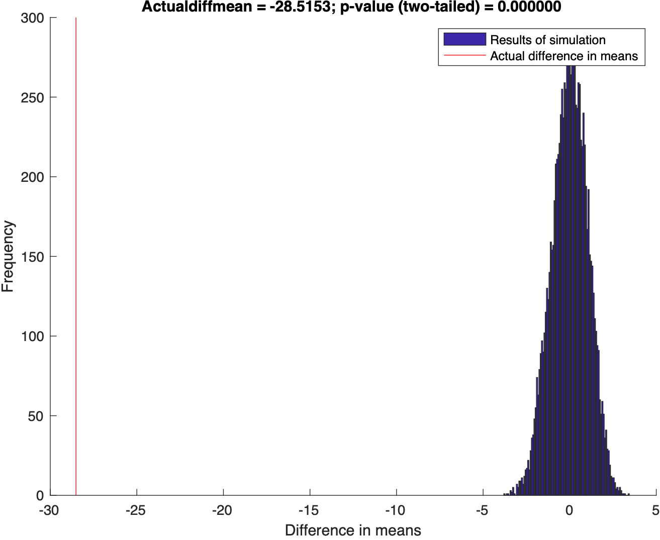
plot(repmat(actualdiffmn,[1 2]),ax(3:4),'r-');
pval = sum(abs(diffmn) > abs(actualdiffmn)) / length(diffmn);
title(sprintf('Actualdiffmean = %.4f; p-value (two-tailed) = %.6f',actualdiffmn,pval));
legend('Results of simulation','Actual difference in means')
xlabel('Difference in means'), ylabel('Frequency')
actualdiffmn =
  -28.5153
MATLAB note: the code uses hist(diffmn,100), which still runs but is legacy — current MATLAB recommends histogram(diffmn,100) (better default binning). The randomization logic is unchanged.
Quick check: The simulation returns a two-tailed p-value of 0.0001 for the observed difference in means. At $\alpha = 0.05$, what’s the right conclusion?
- Accept $H_0$ — the two samples are proven identical
- Reject $H_0$: a difference this large is very unlikely if the samples came from the same population
- Nothing, because randomization tests can’t produce p-values
- Re-run with fewer simulations to raise the p-value
Recap
- State $H_0$ (here: both samples come from one population) and pick a significance level $\alpha$.
- Randomization test: pool the data, shuffle and re-split
numsimtimes withrandperm, and record the statistic (difference in means) each time — this is the null distribution. - The p-value = fraction of shuffled statistics at least as extreme as the observed one (
sum(abs(diffmn) > abs(actualdiffmn))/numsim). - Reject $H_0$ when $p < \alpha$; otherwise fail to reject — which is not the same as proving $H_0$ true (that risks a Type II error).
- This resampling approach needs no Gaussian assumption — it works for any distribution and any statistic.
Where to go next
- Easy statistical analysis in MATLAB — descriptive stats and the classical one-sample t-test.
-
Monte Carlo simulation for correlation — the same simulate-the-null idea applied to a correlation.
- For details see: Lectures on Statistics and Data Analysis in MATLAB (archived)
Found this article useful?
Loading likes…
Disclaimer of liability
The information provided by the Earth Inversion is made available for educational purposes only.
Whilst we endeavor to keep the information up-to-date and correct. Earth Inversion makes no representations or warranties of any kind, express or implied about the completeness, accuracy, reliability, suitability or availability with respect to the website or the information, products, services or related graphics content on the website for any purpose.
UNDER NO CIRCUMSTANCE SHALL WE HAVE ANY LIABILITY TO YOU FOR ANY LOSS OR DAMAGE OF ANY KIND INCURRED AS A RESULT OF THE USE OF THE SITE OR RELIANCE ON ANY INFORMATION PROVIDED ON THE SITE. ANY RELIANCE YOU PLACED ON SUCH MATERIAL IS THEREFORE STRICTLY AT YOUR OWN RISK.
Leave a comment