Plotting track and trajectory of tropical cyclones on a topographic map in Python (codes included)
Loading likes…
Introduction
Plotting track or trajectory of the hurriance is essential part of analyzing and understanding the hurricane. For details see references.
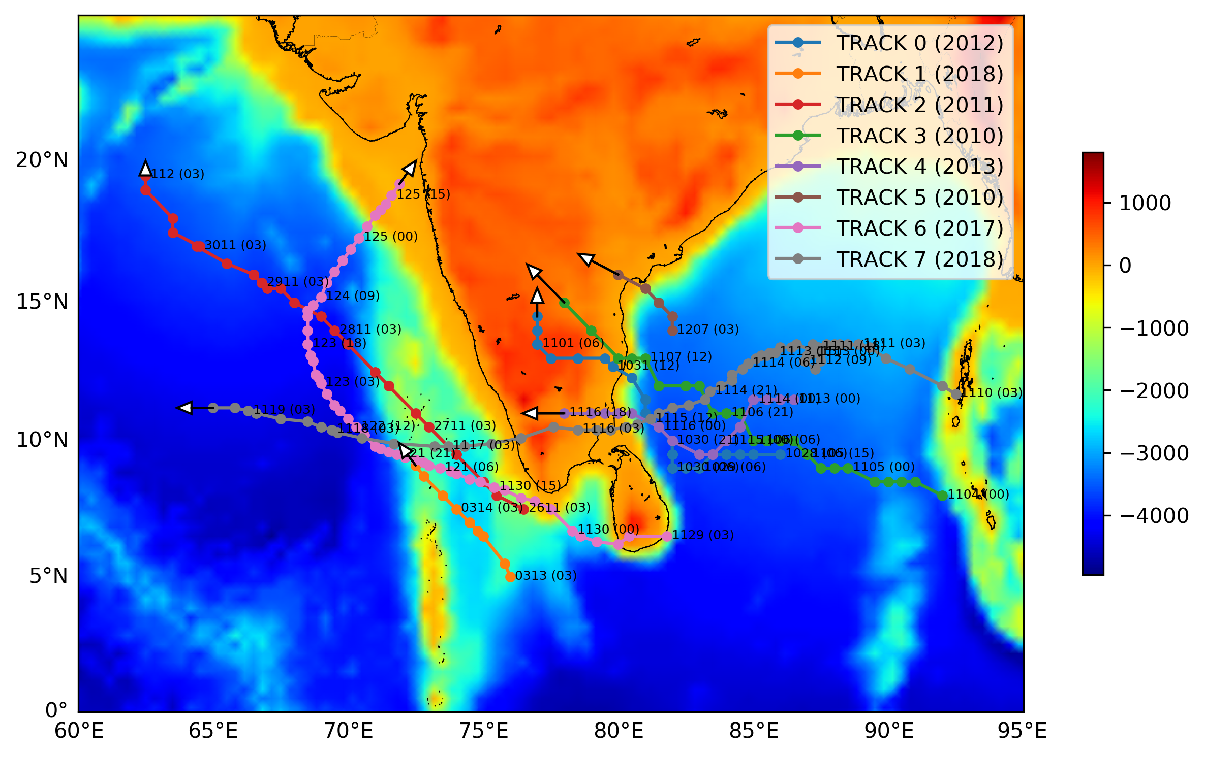
Key idea — a track map is built up in layers. Start with a basemap that fixes the projection and map bounds (here Mercator over the North Indian Ocean), paint the topography underneath, then add reference lines (coastlines, country borders, a lat/lon grid). Only then do you overlay the data: each cyclone’s track is a list of longitude/latitude points that you must first convert to the map’s projected coordinates with x, y = m(lons, lats) before plotting. Finish with annotations — time labels along the path and a direction arrow at the end. Matplotlib’s zorder keeps the stack in order: topography at the bottom, annotations on top.
Basemap is end-of-life (2026 update). mpl_toolkits.basemap had its final release in 2020 and is no longer maintained — its developers now direct users to Cartopy as the supported replacement. The code below still runs where Basemap is installed (via conda install -c conda-forge basemap), and the concepts — projecting coordinates, layering topography and tracks by zorder — carry over directly. For new work, prefer Cartopy or PyGMT; see the companion PyGMT high-resolution topographic map post.
Tropical cyclones (TCs) best track data base sites
- For north Indian Ocean TCs: India Meteorological department
- For south Indian Ocean TCs: Australia bureau of meteorological
- For northwest Pacific TCs: Japan Meteorological Agency
- For Atlantic Ocean: National Oceanic and Atmospheric Administration
- For global tropical cyclones: All oceanic tropical cyclones
Visualization
Importing Libraries
The first thing I like to do is to import all the necessary libraries for the task. This keeps the code organized.
import matplotlib.pyplot as plt
import numpy as np
from mpl_toolkits.basemap import Basemap
import pandas as pd
import glob
from plotting_topo import plot_topo
matplotlib.pyplotis imported for the plotting purpose,numpyis for scientific computation and operations,Basemapis the matplotlib library for plotting 2D data on map,globis for reading the files present in the directory,plot_topois the function that reads the topo data for plotting on the map.
The topo dir is location in the current directory.
Define map boundary parameters
lonmin, lonmax = 60, 95
latmin, latmax = 0, 25
Set up basemap with topography
For more details of plotting topography on a map, see this post for details: How to plot a topographic station map in Python
- instantiate the basemap instance within the defined map boundary. Here, we chose the mercator projection. For other projections, check here
fig = plt.figure(figsize=(10,6))
axx = fig.add_subplot(111)
m = Basemap(projection='merc', resolution="f", llcrnrlon=lonmin, llcrnrlat=latmin, urcrnrlon=lonmax, urcrnrlat=latmax)
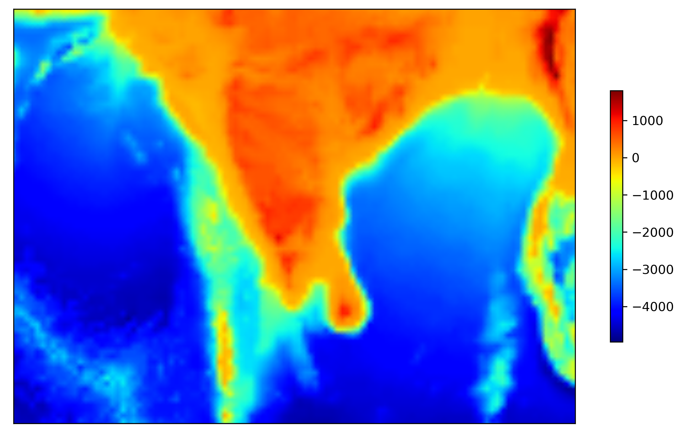
- plot the topography on the basemap and draw colorbar
cs = plot_topo(m,cmap=plt.cm.jet,zorder=2,lonextent=(lonmin, lonmax),latextent=(latmin, latmax))

fig.colorbar(cs, ax=axx, shrink=0.6)
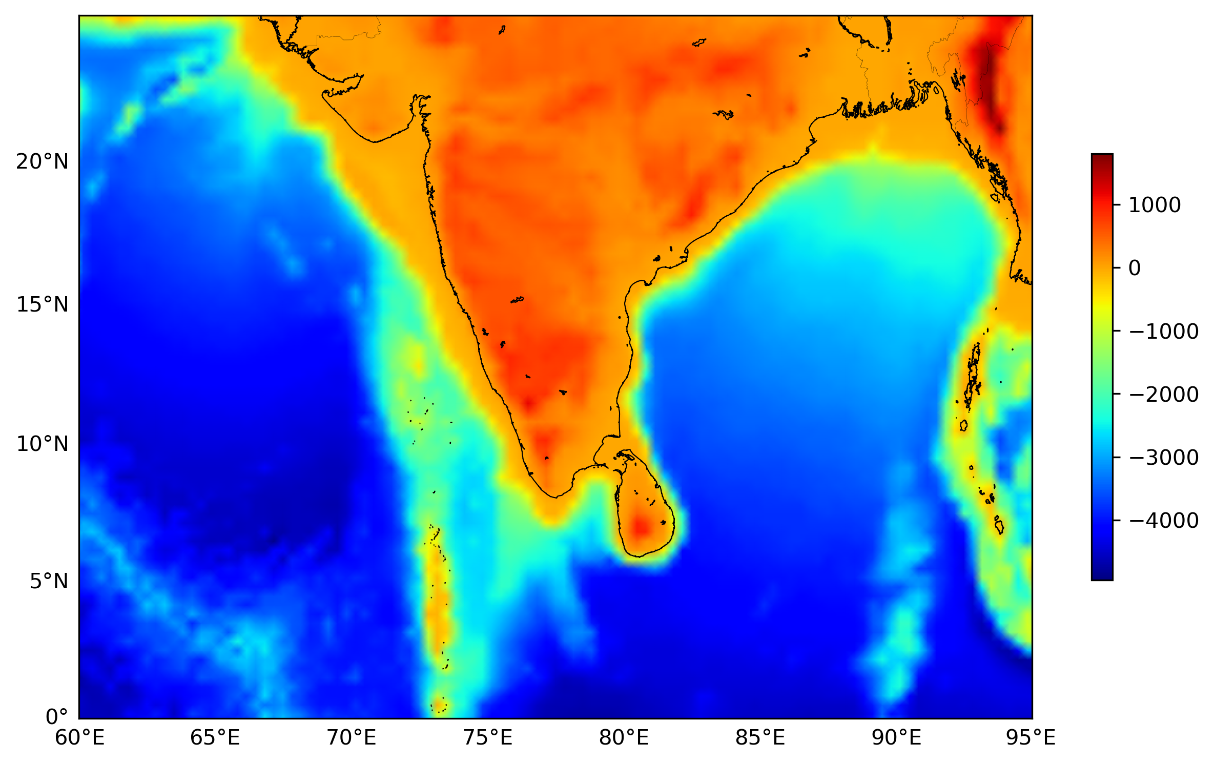
- draw latitudinal and longitudinal grid lines with the step of 5 degrees. We only show the labels on the left and bottom of the map.
m.drawcoastlines(color='k',linewidth=0.5,zorder=3)
m.drawcountries(color='k',linewidth=0.1,zorder=3)

parallelmin = int(latmin)
parallelmax = int(latmax)+1
m.drawparallels(np.arange(parallelmin, parallelmax,5,dtype='int16').tolist(),labels=[1,0,0,0],linewidth=0,fontsize=10, zorder=3)

meridianmin = int(lonmin)
meridianmax = int(lonmax)+1
m.drawmeridians(np.arange(meridianmin, meridianmax,5,dtype='int16').tolist(),labels=[0,0,0,1],linewidth=0,fontsize=10, zorder=3)
Plot track on the basemap
- define the list of colors to be used for different hurriances
- read the file names stored in the directory
01_TRACKS, and with the suffix.txt - read the data file as a pandas data frame.
- extract the
yearinfo from the filename - we “capitalize” the track name
- get longitude and latitude as numpy array
- convert lat and lon to map projection scale
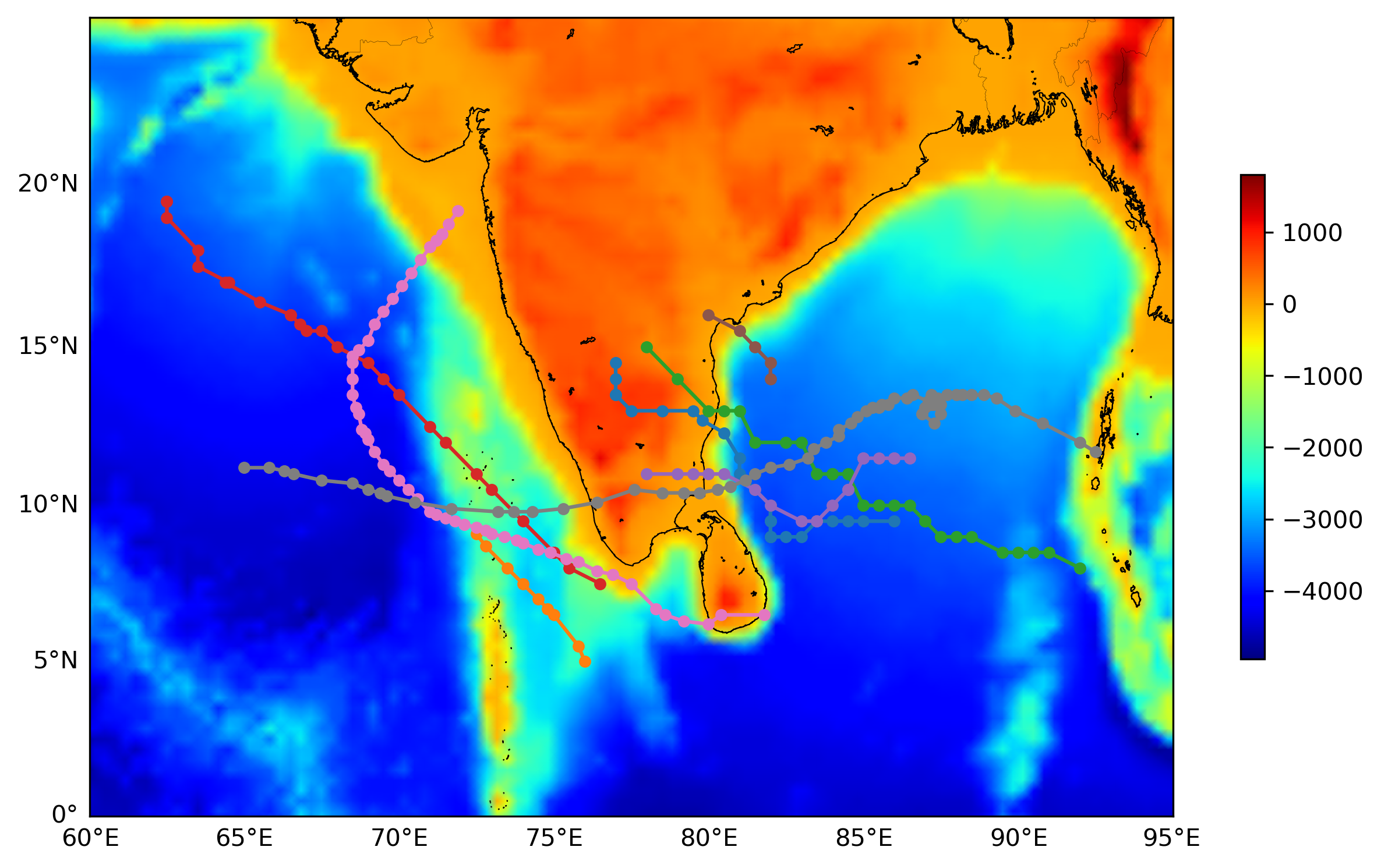
- plot the track with
-oand label the name of each track
colors = ['C0','C1','C3','C2','C4','C5','C6','C7'] #default colors from Python (can be automated if the order is not important)
datafiles = glob.glob("01_TRACKS/*.txt") #to read individual data files containing the coordinates of the track for each typhoon
for jj in range(8):
    dff = pd.read_csv(datafiles[jj],sep='\s+', dtype={'time': object}) #read data file and time as string
    year = datafiles[jj].split("/")[1].split("_")[1].split("-")[0] #extract year information from the filename
    track_name = datafiles[jj].split("/")[1].split("(")[1].split(")")[0] #extract track information from the filename
    track_name = track_name.capitalize()

    ## extract lat and lon info from pandas data frame and convert to map scale
    lons = dff['lon'].values
    lats = dff['lat'].values
    x, y = m(lons, lats)

    ## plot the track
    m.plot(x, y,'o-',color=colors[jj],ms=4, zorder=4,label=f"TRACK {jj} ({year})")
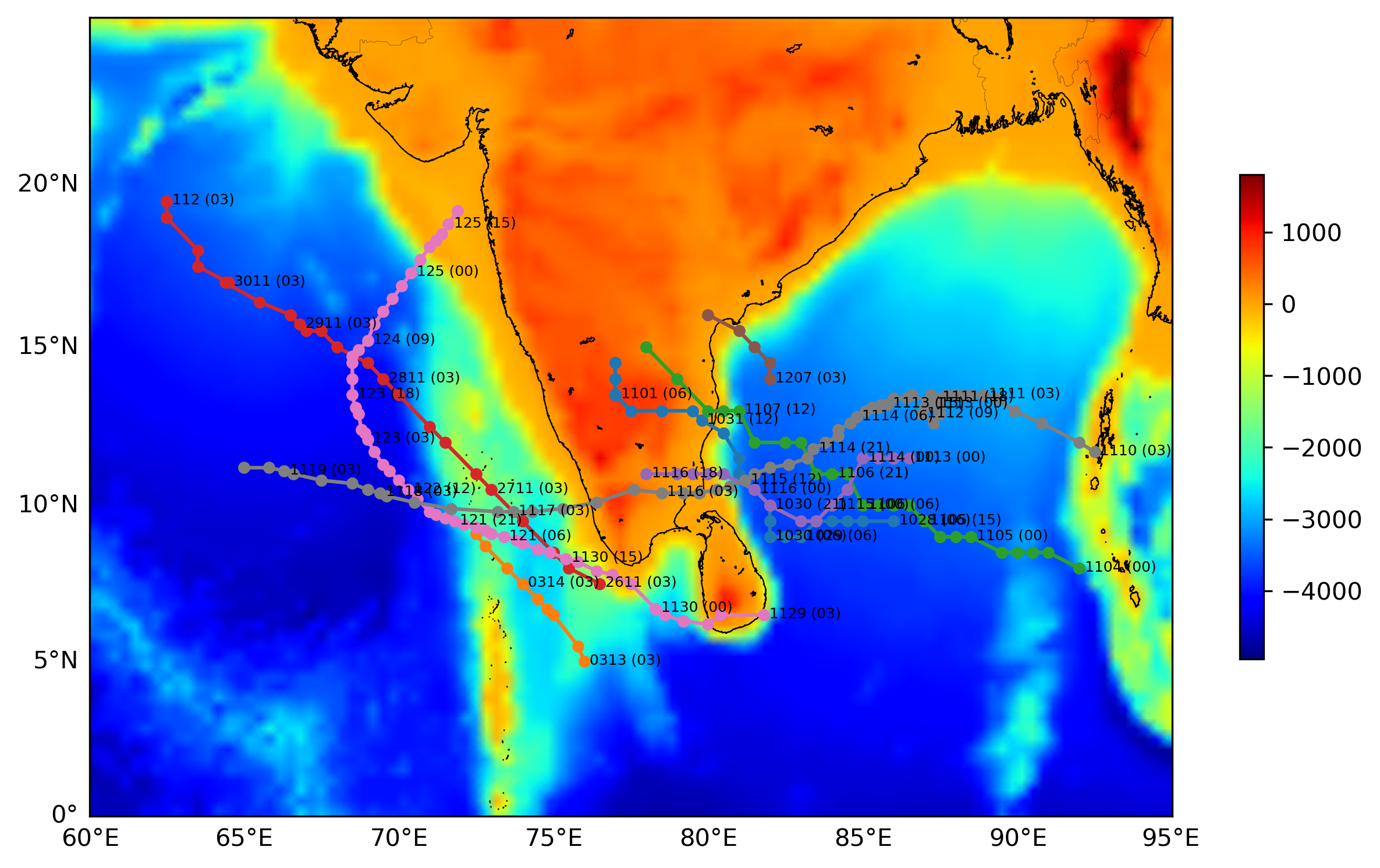
- we extract the time at each data point from the data file for plotting on the map. This gives an idea of the direction of the hurricane.
- the extracted values are the date and month and hour.
- the track time is plotted for every 3rd data point with some shift in x and y direction. The shift is given in terms of the map scale.
for jj in range(8):
  ######CONTINUE FROM ABOVE####
  #############################
    ## extract the time info and label the track with the time for every 3 data points
    typh_time=[]
    for i in range(dff.shape[0]):
        date=dff.loc[i,'date']
        try:
            dd = date.split(".")[0]
            month = date.split(".")[1]
        except:
            dd = date.split("/")[0]
            month = date.split("/")[1]

        time=dff.loc[i,'time']

        track_times="{}{} ({})".format(month, dd, time[:2])
        typh_time.append(track_times)
    typh_time=np.array(typh_time)

    for i in np.arange(0,len(typh_time),5):
        plt.text(x[i]+20000,y[i]-10000,typh_time[i],fontsize=6,zorder=4)
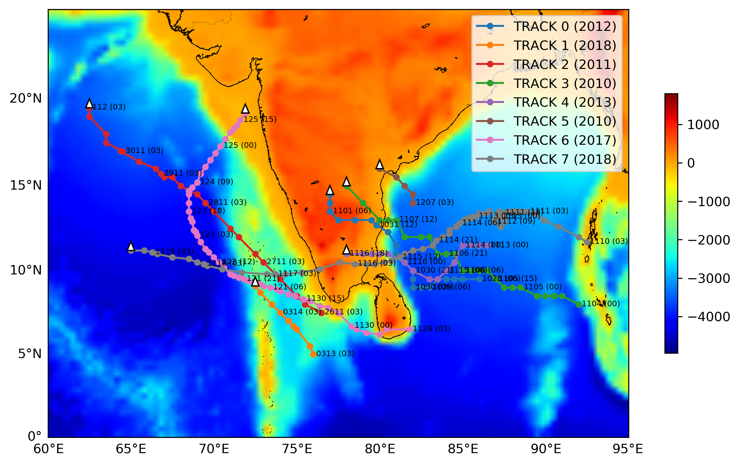
- we can put a triangle at the end of the track to indicate the direction of the hurricane
for jj in range(8):
  ######CONTINUE FROM ABOVE####
  #############################
    ## plot the arrow based on the last two data points to indicate the trajectory of the track
    plt.arrow(x[-1], y[-1]+1, 0, 0,head_width=50000, head_length=60000, fc='w', ec='k',color='k',alpha=1,zorder=4)
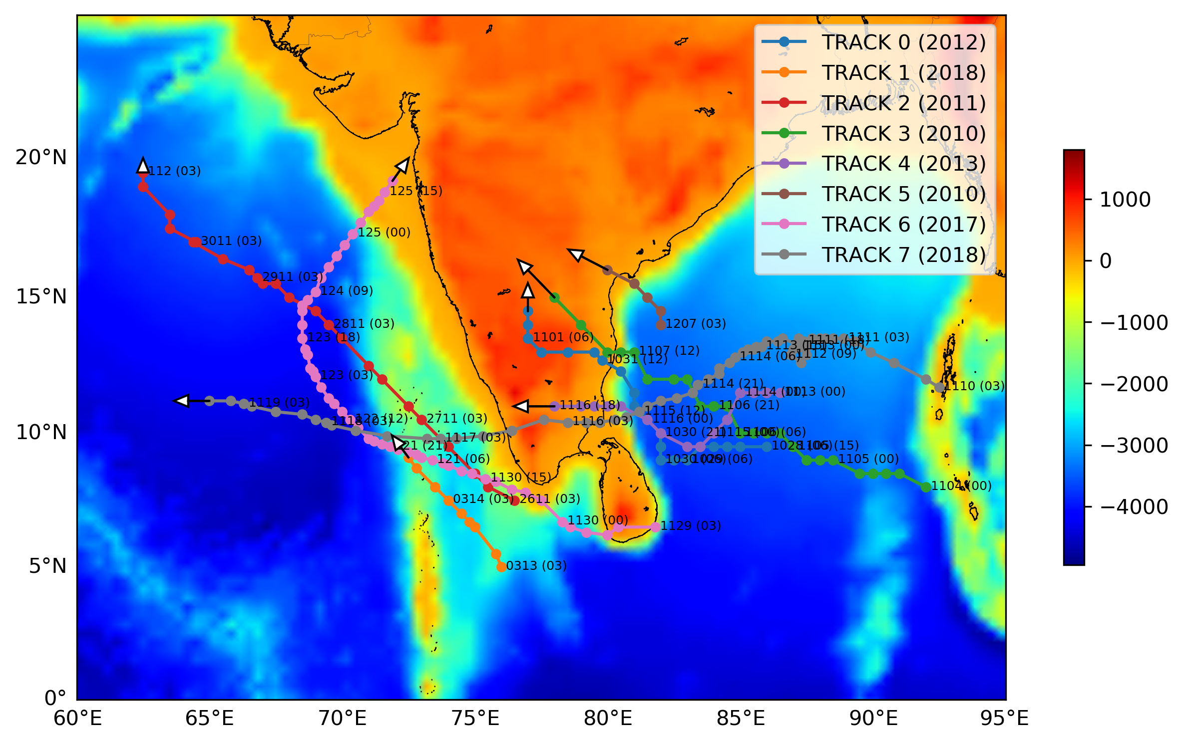
- Instead of just triangle to indicate the direction, we plot the rough trajectory of the hurricane based on the last two data points.
for jj in range(8):
  ######CONTINUE FROM ABOVE####
  #############################
    ## plot the arrow based on the last two data points to indicate the trajectory of the track
    plt.arrow(x[-1], y[-1]+1, x[-1]-x[-2], y[-1]-y[-2],head_width=50000, head_length=60000, fc='w', ec='k',color='k',alpha=1,zorder=4)

plt.legend(loc=1)

## save the map as png
plt.savefig('map.png',bbox_inches='tight',dpi=300)
Quick check: Why does the code call x, y = m(lons, lats) before m.plot(x, y, ...) instead of plotting the raw longitude/latitude directly?
- To convert degrees to radians for matplotlib
- Because
m(...)transforms geographic lon/lat into the Mercator basemap’s projected coordinates, which is whatm.plotexpects - Because pandas stores the values as strings that must be cast to floats
- To reverse the track so the arrow points the right way
Recap
- A track map is a layer stack: basemap (projection + bounds) → topography → coastlines/borders/grid → data (tracks) → annotations, ordered by matplotlib’s
zorder. - Each cyclone’s track is lon/lat points read from a file with
pandas; convert them to the map’s projection withx, y = m(lons, lats)before callingm.plot. - Annotate direction with
plt.texttime labels along the path and aplt.arrowextrapolated from the last two points. - Best-track data comes from the regional RSMCs listed above (IMD, JMA, NOAA/NHC, BoM, JTWC) — each basin has its own agency.
- Basemap is EOL; the same layering logic maps directly onto Cartopy or PyGMT for new projects.
Where to go next
- Plot a high-resolution topographic map with PyGMT — the maintained, publication-quality way to make the basemap layer.
- How to plot a topographic station map in Python — the topography-on-a-map workflow this post builds on.
- Get started with pandas for Earth-data analysis — reading and slicing the track data files.
References
Fovell, R. G., & Su, H. (2007). Impact of cloud microphysics on hurricane track forecasts. Geophysical Research Letters, 34(24), Article L24810. https://doi.org/10.1029/2007GL031723
Huang, Y.-H., Wu, C.-C., & Wang, Y. (2011). The influence of island topography on typhoon track deflection. Monthly Weather Review, 139(6), 1708–1727. https://doi.org/10.1175/2011MWR3560.1
Janapati, J., Seela, B. K., Lin, P.-L., Wang, P. K., & Kumar, U. (2019). An assessment of tropical cyclones rainfall erosivity for Taiwan. Scientific Reports, 9(1), Article 15862. https://doi.org/10.1038/s41598-019-52028-5
Janapati, J., Seela, B. K., Lin, P.-L., Wang, P. K., Tseng, C.-H., Reddy, K. K., Hashiguchi, H., Feng, L., Das, S. K., & Unnikrishnan, C. K. (2020). Raindrop size distribution characteristics of Indian and Pacific Ocean tropical cyclones observed at India and Taiwan sites. Journal of the Meteorological Society of Japan. Ser. II, 98(2), 299–317. https://doi.org/10.2151/jmsj.2020-015
Janapati, J., Seela, B. K., Reddy, M. V., Reddy, K. K., Lin, P.-L., Rao, T. N., & Liu, C.-Y. (2017). A study on raindrop size distribution variability in before and after landfall precipitations of tropical cyclones observed over southern India. Journal of Atmospheric and Solar-Terrestrial Physics, 159, 23–40. https://doi.org/10.1016/j.jastp.2017.04.011
This post was last modified at 2026-10-21 00:39.
Found this article useful?
Loading likes…
Disclaimer of liability
The information provided by the Earth Inversion is made available for educational purposes only.
Whilst we endeavor to keep the information up-to-date and correct. Earth Inversion makes no representations or warranties of any kind, express or implied about the completeness, accuracy, reliability, suitability or availability with respect to the website or the information, products, services or related graphics content on the website for any purpose.
UNDER NO CIRCUMSTANCE SHALL WE HAVE ANY LIABILITY TO YOU FOR ANY LOSS OR DAMAGE OF ANY KIND INCURRED AS A RESULT OF THE USE OF THE SITE OR RELIANCE ON ANY INFORMATION PROVIDED ON THE SITE. ANY RELIANCE YOU PLACED ON SUCH MATERIAL IS THEREFORE STRICTLY AT YOUR OWN RISK.
Leave a comment