GMT tutorial for beginners (codes included)
Loading likes…
The Generic Mapping Tools is widely used across Earth and Planetary and other fields of studies to process data and generate high quality illustrations. This post is first introduction to beginners for getting started in GMT.
Please note that recently GMT version 6 has been released but this post is focussed on GMT version 5. For readers interested in GMT 6, I recommend beginners to get started with pyGMT.
Key idea — a GMT map is built by layering commands. Every GMT figure starts by fixing the region (-R) and projection (-J), then stacks layers on top: a frame (-B), coastlines, data points (psxy), contours (grdcontour), a colorbar (psscale). The examples below use GMT 5 classic mode, where each ps* command appends to a single PostScript file and you thread them together with -K (“more layers coming”) and -O (“overlay”). GMT 6’s modern mode wraps the same idea in gmt begin … gmt end and drops that bookkeeping — but the mental model (region → projection → layers) is identical.
gmt begin … gmt end.GMT 5 is old — the current release is GMT 6.6. This tutorial targets GMT 5 classic mode, which still runs, but GMT has been on the 6.x series for years (latest 6.6.0) with modern mode as the recommended interface: the ps* commands became basemap/coast/plot, -K/-O are gone, and figures are wrapped in gmt begin … gmt end. See the companion post on the modern interface to GMT, or drive GMT 6 from Python with PyGMT. The concepts and projections below carry straight over.
How to install GMT
In Ubuntu: sudo apt-get install gmt gmt-dcw gmt-gshhg
In Mac: brew install gmt
For other operating systems, check the GMT download page
Requirements:
Below is a list of examples, originally inspired from the GMT documentation. For successfully running the codes, the user need to fulfill following requirements:
- Pre-installed GMT-5, check by typing
gmtin terminal. - Pre-installed netcdf-5, check by typing
ncdump. - Pre-installed ghostview package, check by typing
gv. - Downloaded
ETOPO1_Bed_g_gmt4.grdin the Data directory from the NOAA website.
Examples:
Readers can download the package containing all the following examples from here. The package consists of three directories: Data, Scripts and Figures.
- The Data directory contains the data files required to run the scripts in the Scripts directory.
- The Scripts directory consists of all the bash scripts for all the later examples.
- The Figures directory consists of all the example plots from 1-24.
Linear Plots
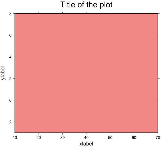
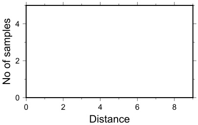
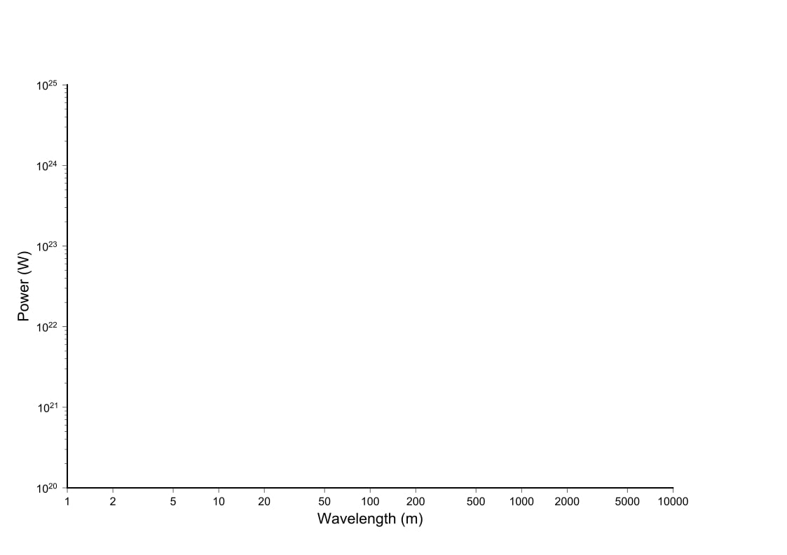
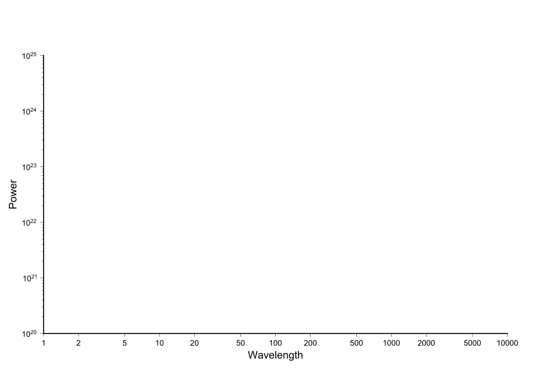
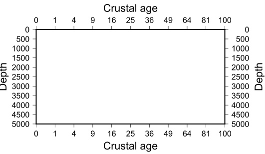
This script contains commands for making basemap for linear projections including the log-log plot. It also explains how to add title, xlabel, ylabel, tick-marks, background-color to the plot.
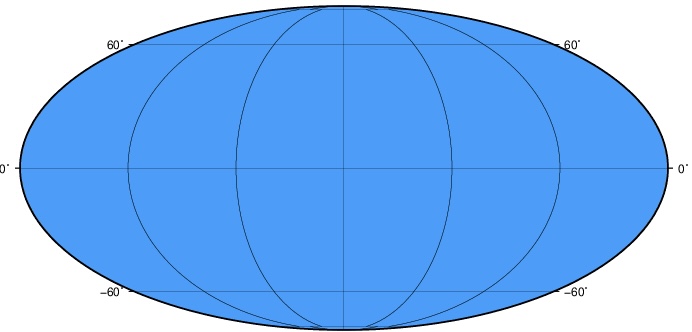
Plotting maps with different projections
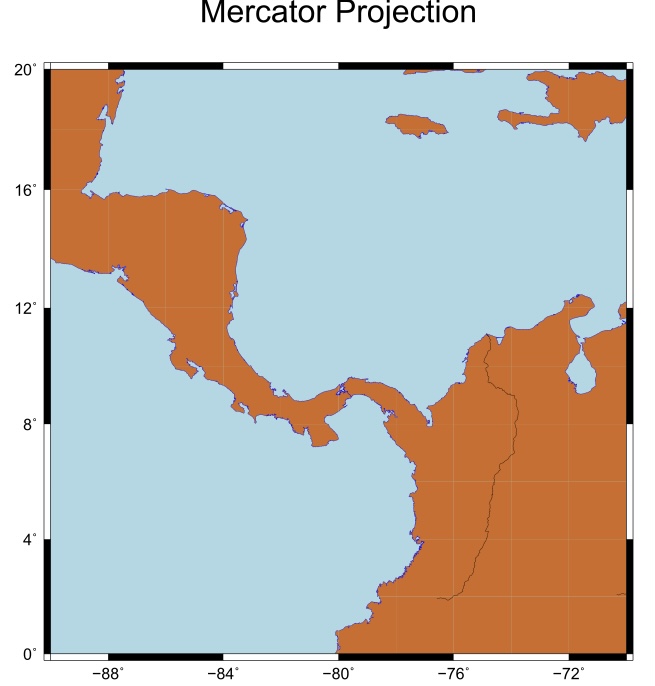
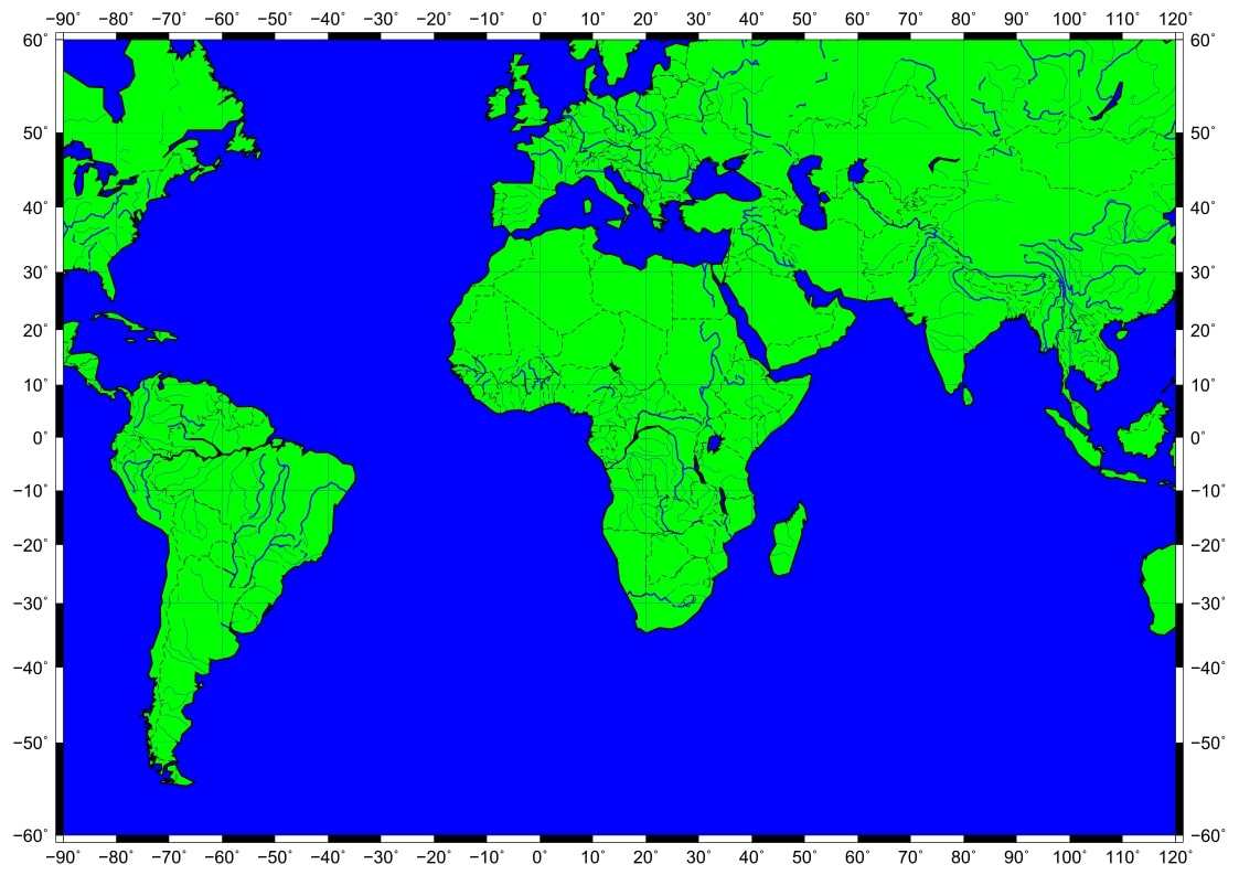
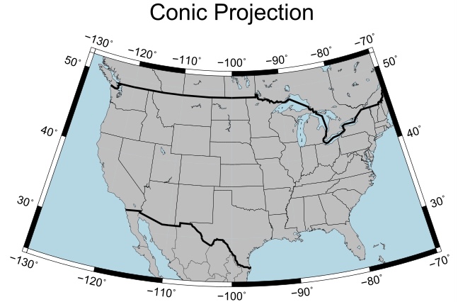
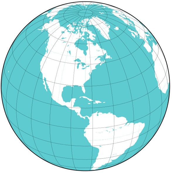
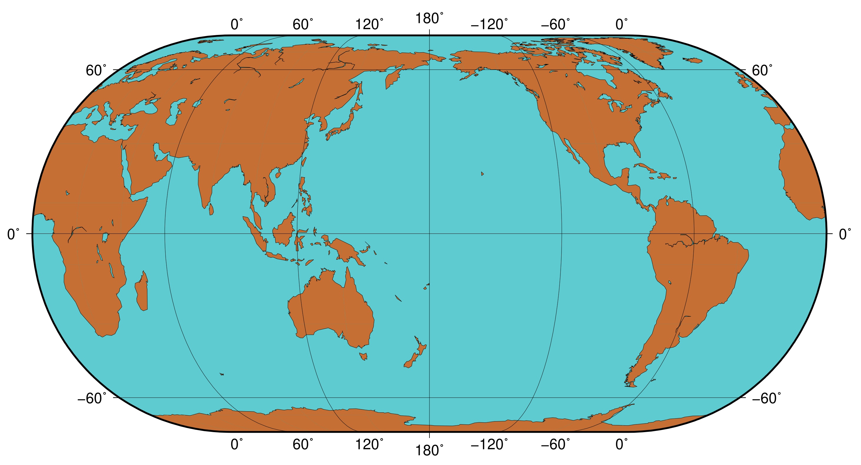
This example explains how to plot the Mercator projection, Alber’s projection, Orthographic projection, Eckert projection.
Plotting lines and symbols
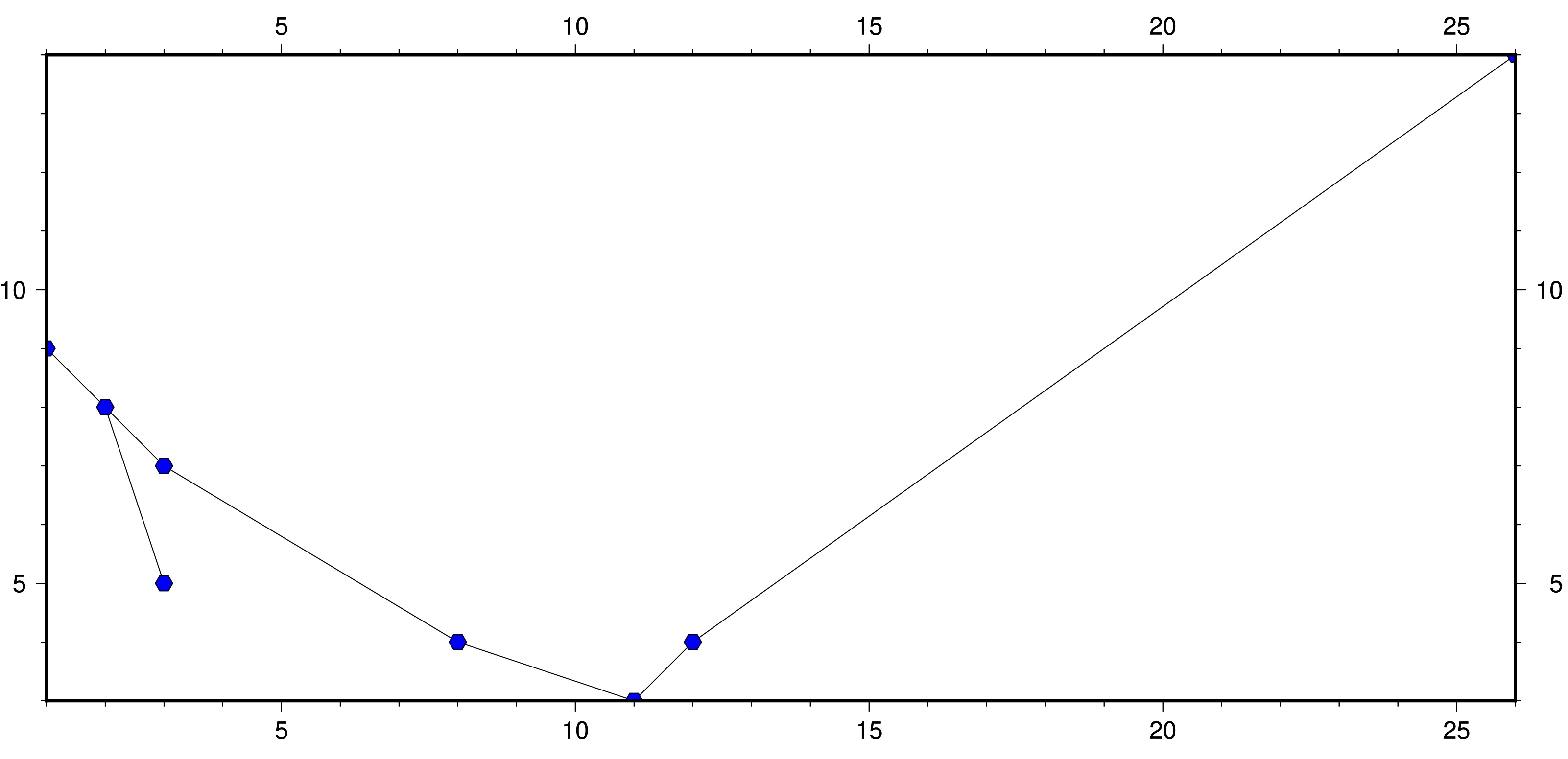
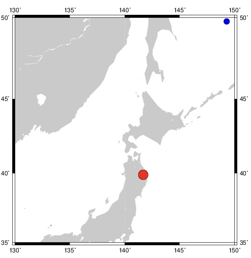
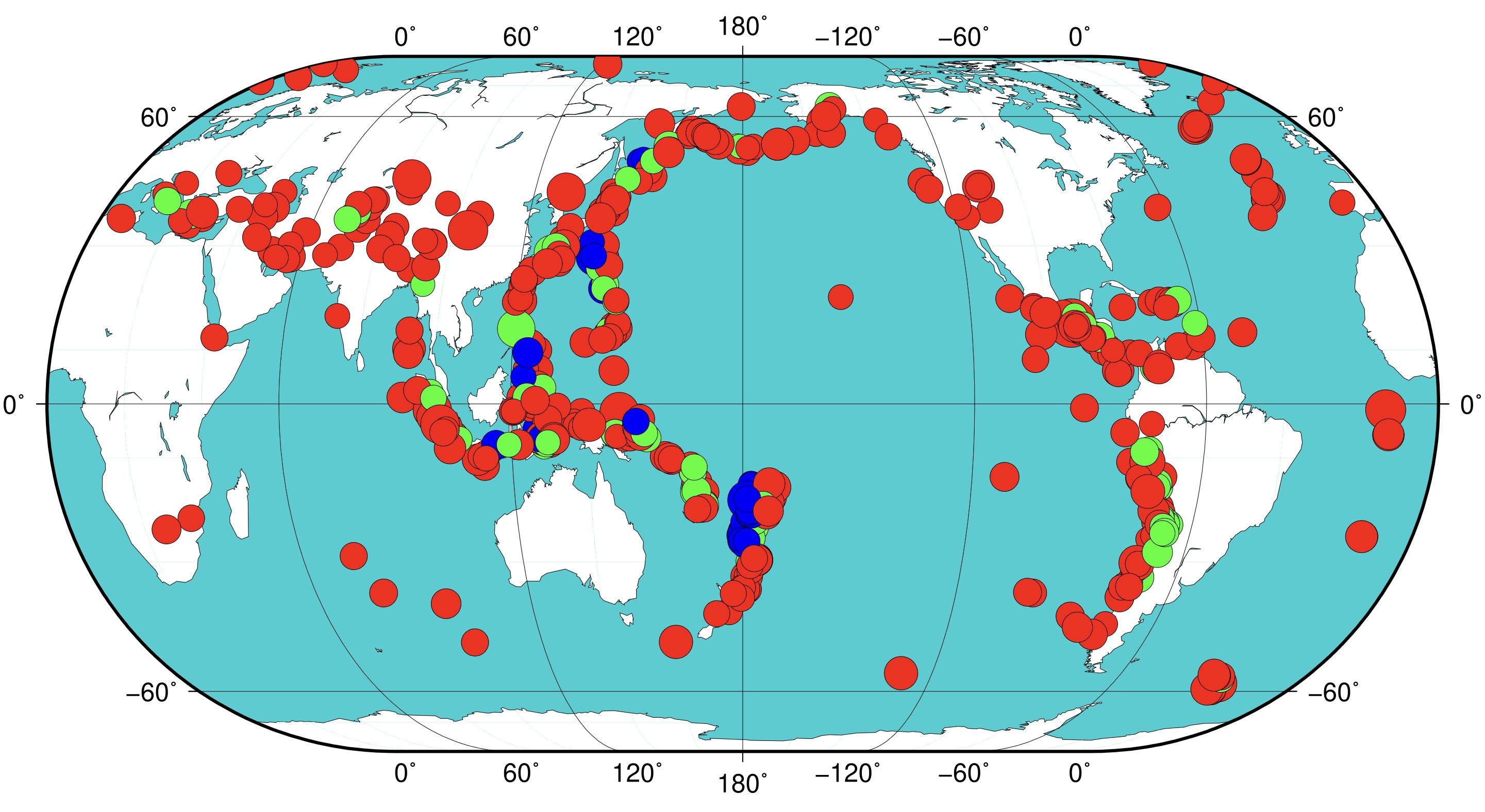
This example explains the use of psxy command to plot the lines and symbols. It also contains the commands to plot the earthquake epicenter with colors representing depths and symbol size representing magnitude.
Customizing plots with texts
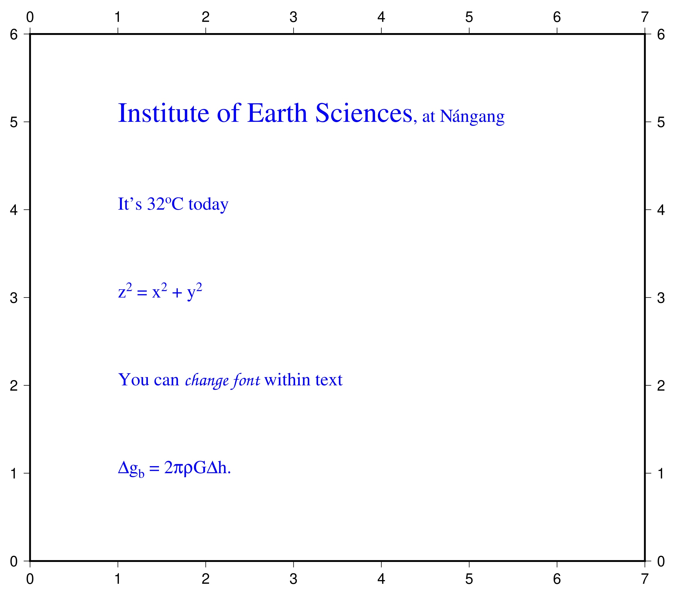
This example explains how to type texts onto the plots. The user can even type mathematical equations.
Contour lines in GMT
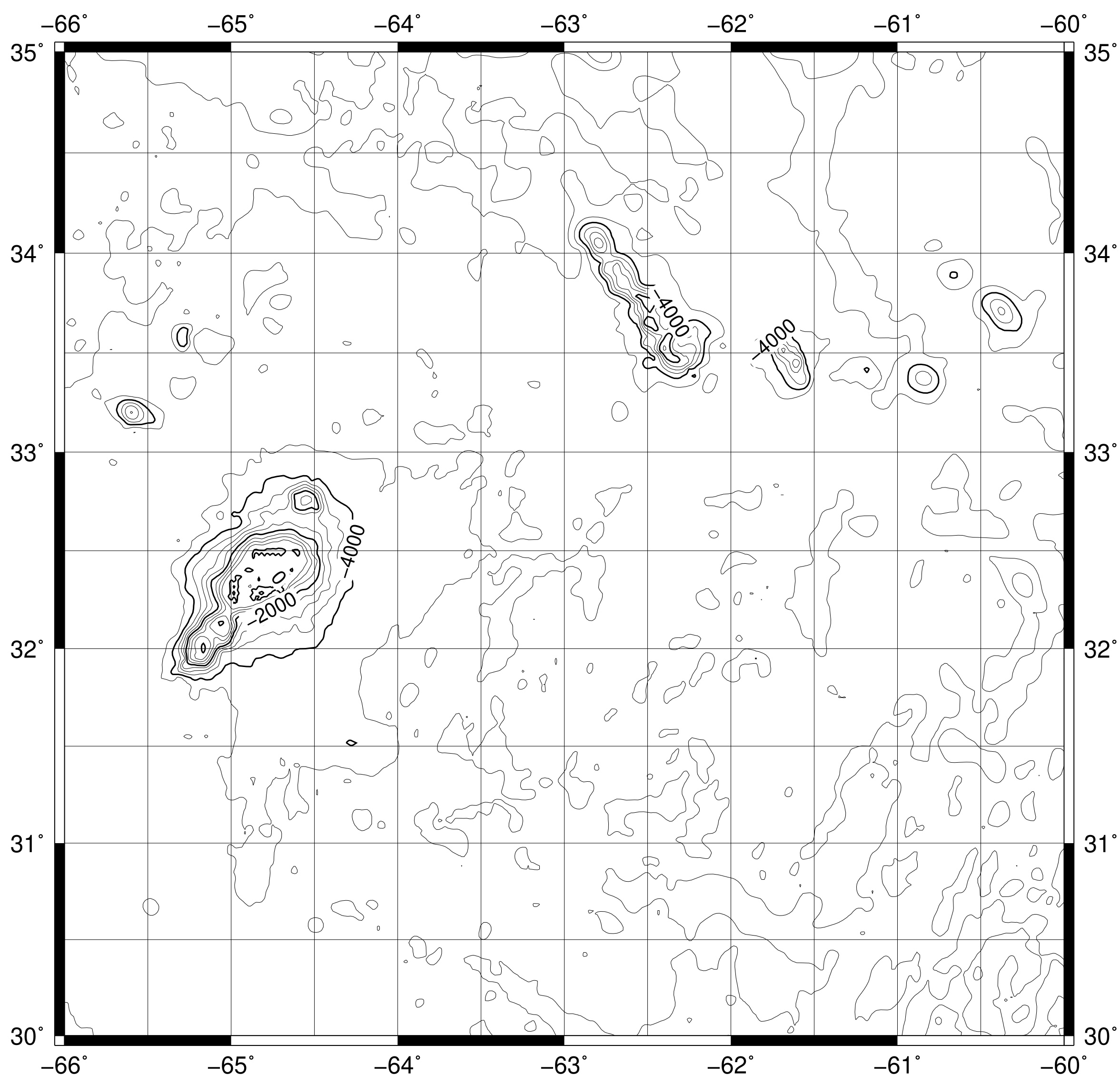
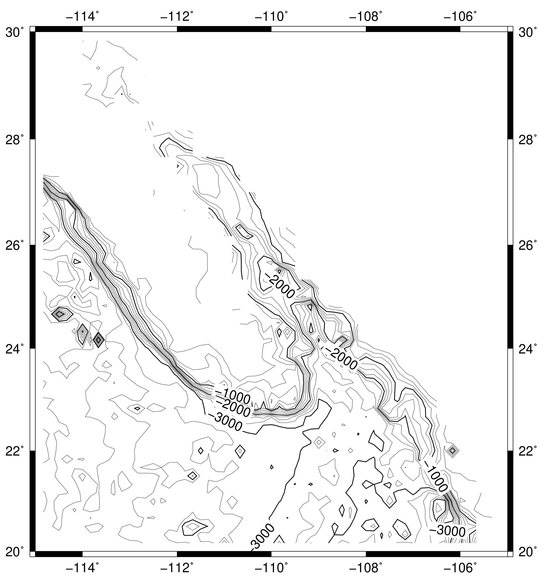
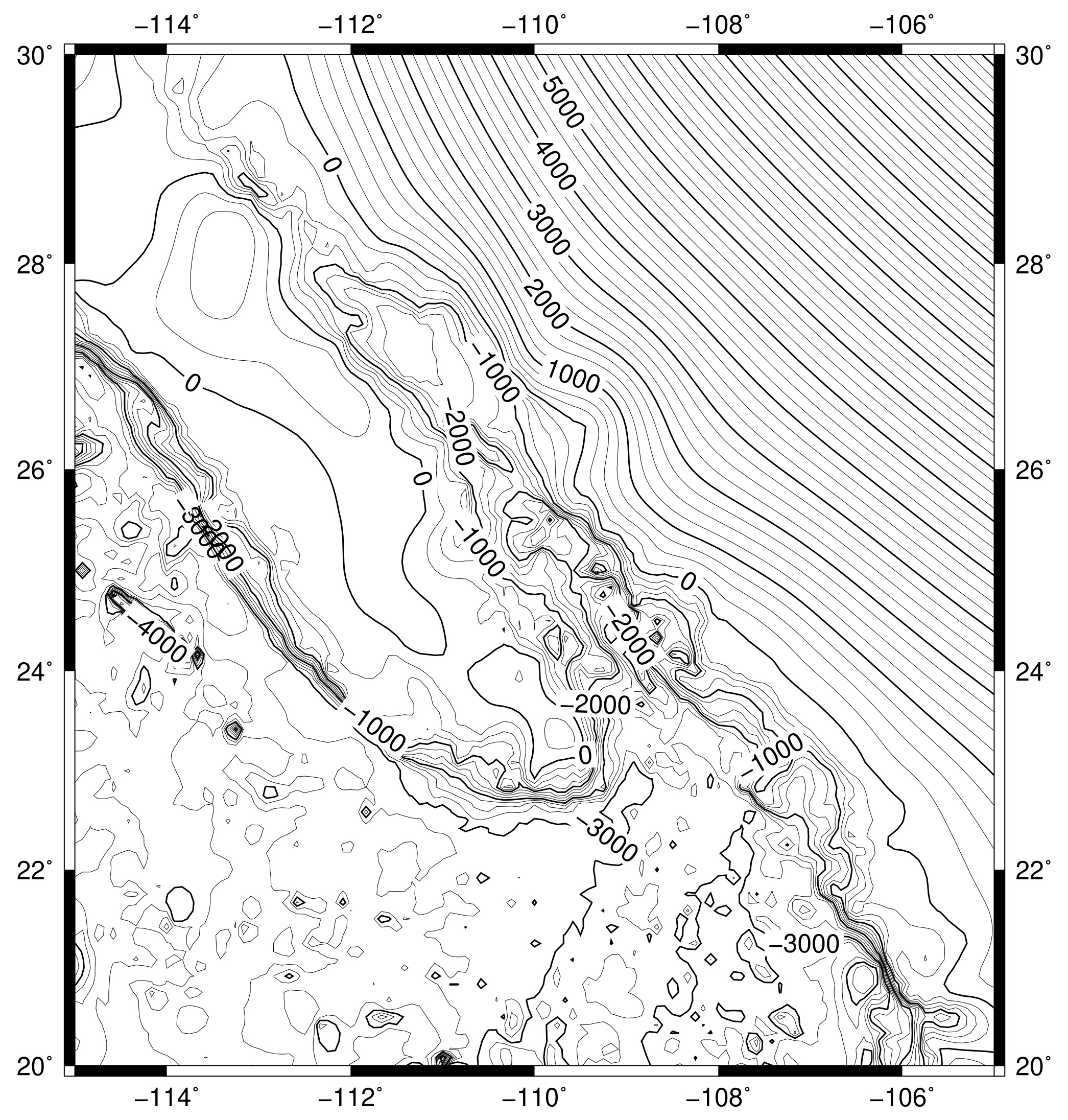
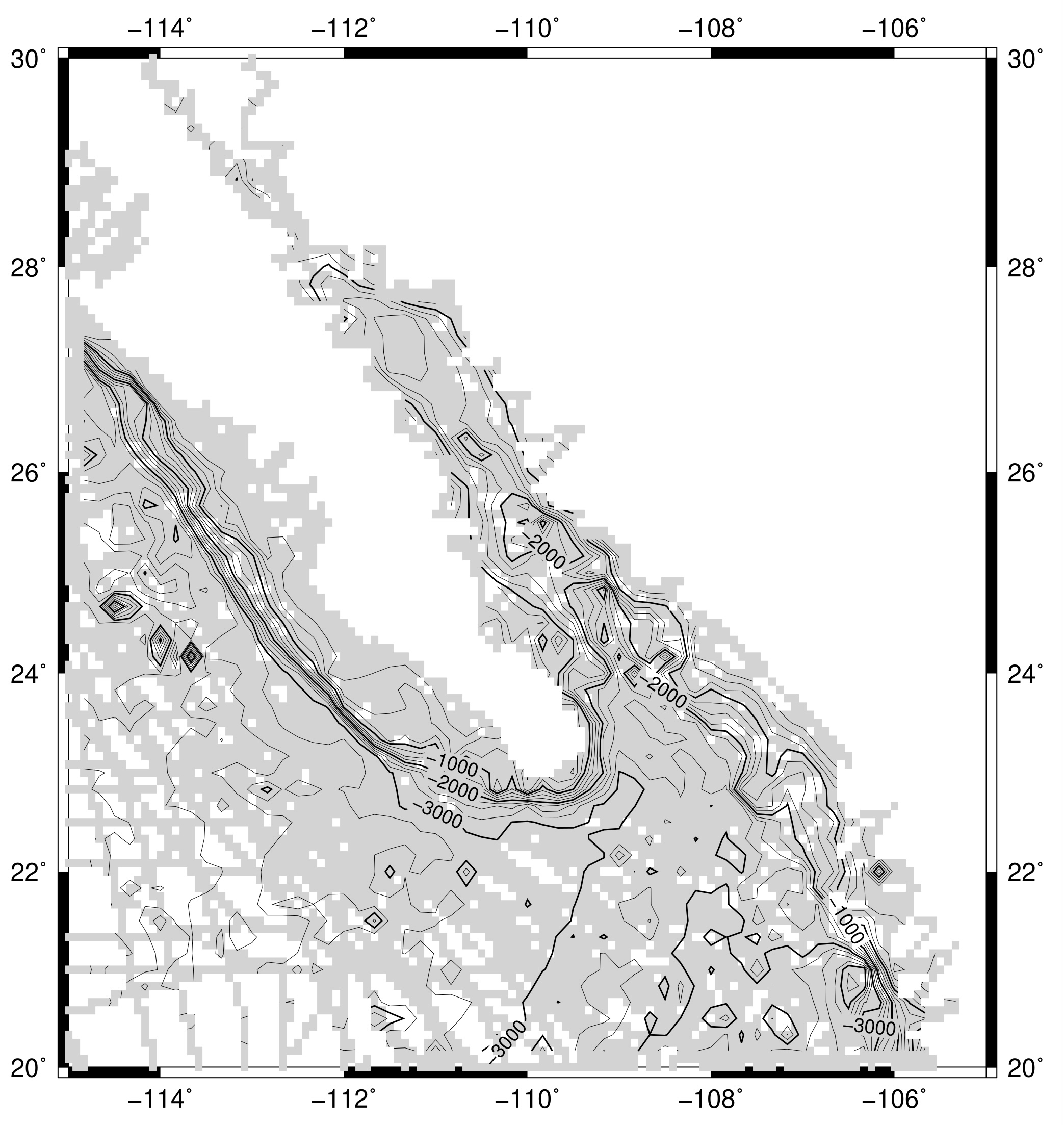
This bash example explains how to plot the contour lines using the command grdcontour. It also explains how to cut the large data set using the grdcut command and obtain the information about it using the grdinfo. It also explains how to do interpolation of data (nearest neighbour and spline).
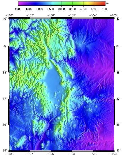
Colorbars and colorscales
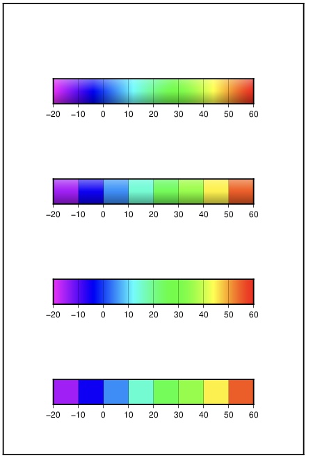
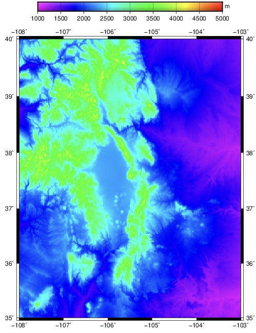
This example contains the description of how to make the cpt files, and plot the colorbars using psscale command. It also explains plotting the relief data.
Plotting NetCDF data in GMT
This example shows how to plot the multidimensional netcdf data in GMT.
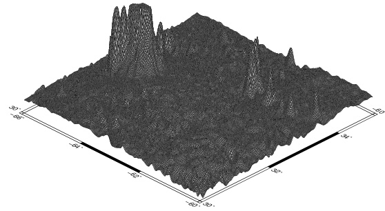
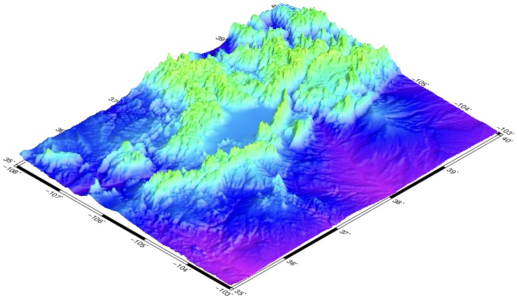
Three dimensional plots: Mesh and Surface plots
This examples script includes how to plot the data as 3D plots using two methods: mesh plot, color-coded surface.
Quick check: In GMT 5 classic mode, what do the -K and -O flags do?
- They set the map’s colour and opacity
- They chain PostScript layers —
-Ksays “more layers follow” and-Osays “overlay onto the existing file” - They control the output resolution
- They are required only for 3-D plots
Recap
- Every GMT figure is built the same way: set the region (
-R) and projection (-J), then layer on a frame (-B), coastlines, data (psxy), contours (grdcontour), and a colorbar (psscale). - These examples use GMT 5 classic mode, where
ps*commands append to a PostScript file and-K/-Othread the layers together, followed bypsconvertto a raster image. - The tutorial covers the essentials: linear/log basemaps, projections (Mercator, Albers, Orthographic, Eckert), lines and symbols, text/equations, contours and interpolation, colorbars and CPTs, NetCDF grids, and 3-D mesh/surface plots.
- GMT 5 is legacy — the maintained release is GMT 6.6 with modern mode (
gmt begin/gmt end, no-K/-O); the concepts transfer directly.
Where to go next
- High-quality maps with the modern interface to GMT — the GMT 6 modern-mode version of this material.
- PyGMT: high-resolution topographic maps in Python — drive GMT 6 from Python.
- Three-dimensional perspective map of Taiwan (GMT & PyGMT) — go further with 3-D relief.
Found this article useful?
Loading likes…
Disclaimer of liability
The information provided by the Earth Inversion is made available for educational purposes only.
Whilst we endeavor to keep the information up-to-date and correct. Earth Inversion makes no representations or warranties of any kind, express or implied about the completeness, accuracy, reliability, suitability or availability with respect to the website or the information, products, services or related graphics content on the website for any purpose.
UNDER NO CIRCUMSTANCE SHALL WE HAVE ANY LIABILITY TO YOU FOR ANY LOSS OR DAMAGE OF ANY KIND INCURRED AS A RESULT OF THE USE OF THE SITE OR RELIANCE ON ANY INFORMATION PROVIDED ON THE SITE. ANY RELIANCE YOU PLACED ON SUCH MATERIAL IS THEREFORE STRICTLY AT YOUR OWN RISK.
Leave a comment