PyGMT: High-Resolution Topographic Map in Python (codes included)

If you have worked in seismology, you have almost certainly met Generic Mapping Tools (GMT) — the free, open-source engine behind countless publication-quality maps across the Earth, ocean, and planetary sciences. PyGMT is its modern Python wrapper, so you get GMT’s cartographic power with the convenience of a Python script. In this tutorial we build a topographic map of southern India from scratch and drop a few markers on it.

The single most useful mental model for PyGMT is this: a figure is a stack of layers. You create a blank Figure, then each command (grdimage, coast, grdcontour, plot, colorbar) paints one more layer on top. Once that clicks, the rest is just looking up options.

Setup: install PyGMT

PyGMT needs the GMT C library underneath it, so the maintainers recommend installing it with conda/mamba, which pulls in GMT for you:

conda install --channel conda-forge pygmt

Set up the problem

Import the libraries and define the geographic box we want to map. We import numpy here because we will use it later to generate some sample point coordinates.

import pygmt
import numpy as np

minlon, maxlon = 60, 95
minlat, maxlat = 0, 25

Choose a topographic data source

GMT can stream global relief grids on demand — you just name the grid and it downloads and caches the tiles. The trailing code sets the resolution:

# define the relief grid (downloaded and cached automatically)
# topo_data = 'path_to_local_data_file'   # or point to your own grid
topo_data = '@earth_relief_30s'  # 30 arc-second global relief (SRTM15+V2.1, ~1 km)
# topo_data = '@earth_relief_15s'  # 15 arc-second global relief (SRTM15+V2.1)
# topo_data = '@earth_relief_03s'  # 3 arc-second global relief (SRTM3, ~90 m)

Build the map, one layer at a time

Start a figure

Just like matplotlib’s fig = plt.figure(), every PyGMT map begins with a Figure instance.

fig = pygmt.Figure()

Define a color palette (CPT)

makecpt builds the color palette that grdimage will use to color elevations. Here elevations run from −8000 m to +8000 m in 1000 m steps using GMT’s built-in topo palette.

pygmt.makecpt(
    cmap='topo',
    series='-8000/8000/1000',
    continuous=True
)

Paint the relief

Now we draw the relief image itself. We pass the grid, the region ([minlon, maxlon, minlat, maxlat]), and a projection. You can also give region as an ISO country code — e.g. IN for India, TW for Taiwan (see the ISO code list). Here projection='M4i' means a 4-inch-wide Mercator map (more options in the GMT projection reference).

fig.grdimage(
    grid=topo_data,
    region=[minlon, maxlon, minlat, maxlat],
    projection='M4i'
)

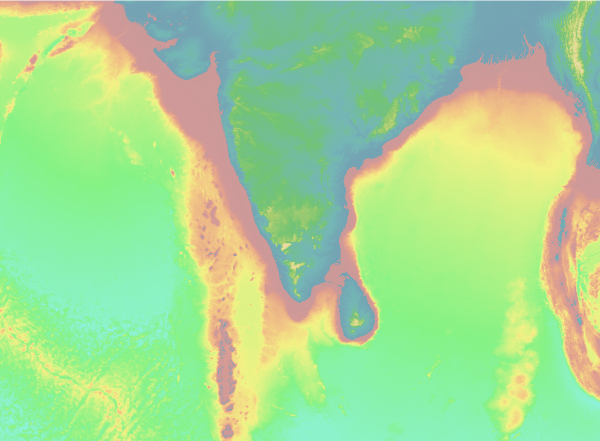
Add frame=True to draw the map frame with automatic tick marks and labels:

fig.grdimage(
    grid=topo_data,
    region=[minlon, maxlon, minlat, maxlat],
    projection='M4i',
    frame=True
)

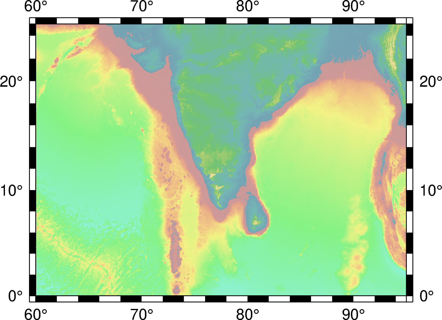
Now add shading=True. This simulates illumination from the side, giving the terrain a three-dimensional, hill-shaded look:

fig.grdimage(
    grid=topo_data,
    region=[minlon, maxlon, minlat, maxlat],
    projection='M4i',
    shading=True,
    frame=True
)

Add coastlines

fig.coast draws continents, shorelines, rivers, and borders. Full options are in the pygmt.Figure.coast docs.

fig.coast(
    region=[minlon, maxlon, minlat, maxlat],
    projection='M4i',
    shorelines=True,
    frame=True
)

Add topographic contours

Contour lines emphasize how the elevation changes. Here we contour every 4000 m and, with limit="-8000/0", show only the sub-sea-level (bathymetry) contours.

fig.grdcontour(
    grid=topo_data,
    interval=4000,
    annotation="4000+f6p",
    limit="-8000/0",
    pen="a0.15p"
)

Plot data points

Now we drop some markers. We generate ten random coordinates inside our region (this is why we imported numpy) and plot them as red circles.

# generate sample coordinates inside the region
lons = minlon + np.random.rand(10) * (maxlon - minlon)
lats = minlat + np.random.rand(10) * (maxlat - minlat)

# plot the points as red circles
fig.plot(
    x=lons,
    y=lats,
    style='c0.1i',   # circles, 0.1 inch
    fill='red',
    pen='black',
    label='something'
)

Change style to use any GMT symbol — for example a0.1i draws 0.1-inch stars instead of circles.

Add a colorbar

By default the colorbar is horizontal:

fig.colorbar(
    frame='+l"Topography"'
)

For a vertical colorbar, set its position explicitly — the +v at the end requests the vertical orientation:

fig.colorbar(
    frame='+l"Topography"',
    position="x11.5c/6.6c+w6c+jTC+v"
)

Show and save the figure

Like matplotlib, PyGMT previews the figure with fig.show():

fig.show()  # fig.show(method='external') opens it in an external viewer

To save it, use fig.savefig. PyGMT crops the figure by default and exports at 300 dpi for PNG and 720 dpi for PDF, among other formats:

fig.savefig("topo-plot.png", crop=True, dpi=300, transparent=True)

fig.savefig("topo-plot.pdf", crop=True, dpi=720)

To export several formats at once:

allformat = 1

if allformat:
    fig.savefig("topo-plot.pdf", crop=True, dpi=720)
    fig.savefig("topo-plot.eps", crop=True, dpi=300)
    fig.savefig("topo-plot.tif", crop=True, dpi=300, anti_alias=True)

The complete script

Going further

The three sections below are self-contained extensions. They are more advanced, so they are tucked into expandable panels — open the one you need.

   stn1     stlo1    stla1  stn2     stlo2    stla2
0  A002  121.4669  25.1258  B077  120.7874  23.8272
1  A002  121.4669  25.1258  B117  120.4684  24.1324
2  A002  121.4669  25.1258  B123  120.5516  24.0161
3  A002  121.4669  25.1258  B174  120.8055  24.2269
4  A002  121.4669  25.1258  B183  120.4163  23.8759

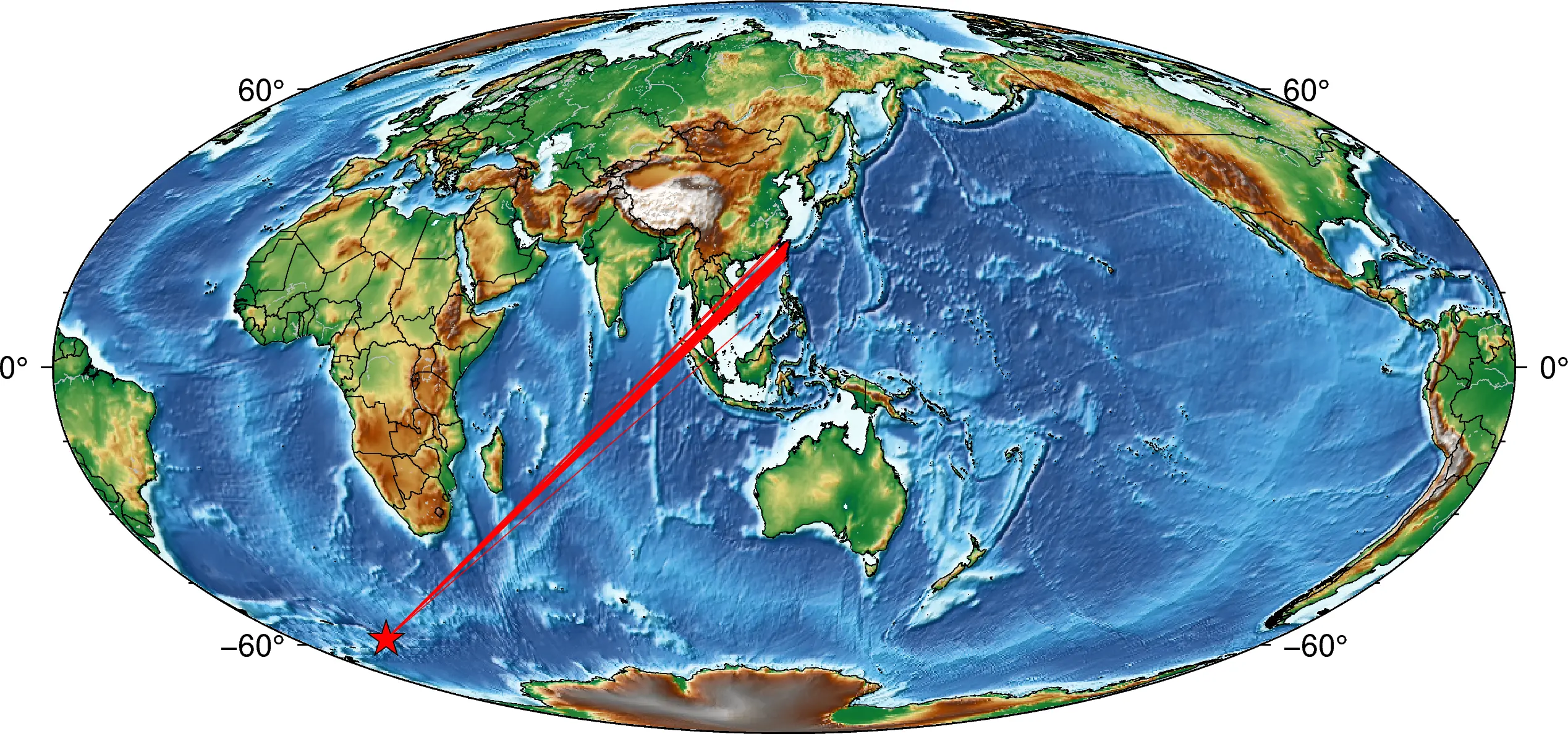
Make an event–station map (Mollweide projection)

This example uses the Mollweide projection, but the code adapts to any projection with a small tweak. The first few lines of the data file look like:

Recap

Without scrolling up, can you name the layers we stacked? You now know how to:

• install PyGMT with conda install -c conda-forge pygmt;
• choose a relief grid at the right resolution (@earth_relief_30s, 03s, …);
• stack the map: makecpt → grdimage (with frame and shading) → coast → grdcontour → plot → colorbar;
• export it at publication DPI with fig.savefig.

That layering pattern is the whole game — every other PyGMT map you make is a variation on it.

Where to go next

• PyGMT API reference and gallery
• A Quick Overview on Geospatial Data Visualization using PyGMT
• How to plot earthquake data on a topographic map

References

1. Uieda, L., Wessel, P., 2019. PyGMT: Accessing the Generic Mapping Tools from Python. AGUFM 2019, NS21B--0813.
2. Wessel, P., Luis, J.F., Uieda, L., Scharroo, R., Wobbe, F., Smith, W.H.F., Tian, D., 2019. The Generic Mapping Tools Version 6. Geochemistry, Geophys. Geosystems 20, 5556–5564. https://doi.org/10.1029/2019GC008515