Efficiently compute spectrogram for large dataset in python
Loading likes…
In previous posts, we have obtained the spectrogram of time series (seismic or otherwise) using mainly two approaches. We first used the Obspy’s spectrogram method to plot the spectrogram for seismic time series (see post 1 and post 2). We have then modified the Obspy’s spectrogram method to customize it to work more efficiently for our purpose (see post). We have also used MATLAB to plot the spectrogram (see here). But for most of the methods we used, we have seen that they suffer to compute the spectrogram for larger time series data. In this post, we will explore another module to compute the spectrogram of the time series.
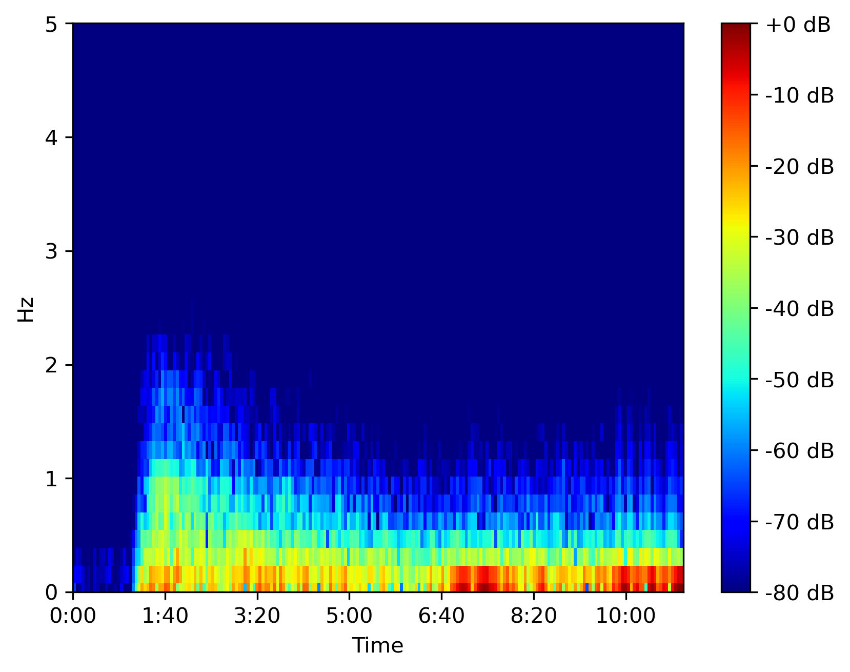
Key idea — a spectrogram is just the FFT taken in short, sliding windows. Rather than one Fourier transform over the whole signal, the short-time Fourier transform (STFT) slides a small window along the data and takes an FFT at each step, producing a 2-D map of how the frequency content changes over time. Two knobs control it: n_fft (window length → frequency resolution) and hop_length (how far the window slides → time resolution). Making the window longer sharpens frequency but blurs time — that time–frequency trade-off is the whole game.
Librosa
Librosa is a Python package designed for music and audio signal analysis. However, we will explore it for analyzing the seismic time series. This package has been designed for the purpose of applying machine learning analysis on the music data. For this sake, the package is required to be very efficient.
Librosa’s spectrogram operations include the short-time Fourier transform (stft), inverse STFT (istft), and instantaneous-frequency spectrogram (ifgram), which provide much of the core functionality for downstream feature analysis. It also provides an efficient constant-Q transform (cqt) — based on the recursive downsampling method of Schörkhuber and Klapuri (2010) — which produces logarithmically-spaced frequency representations suitable for pitch-based analysis. Finally, log-amplitude scaling (amplitude_to_db / power_to_db, which replaced the old logamplitude) converts from linear amplitude to decibels while avoiding numerical underflow and setting an adaptive noise floor. For details, check the references.
For spectrogram analysis, Librosa stores the spectrograms as 2-dimensional numpy arrays, where the first axis is frequency, and the second axis is time.
Parameters used by Librosa
Some of the parameters used by the Librosa for analysis:
sr = sampling rate (Hz), default: 22050
frame = short audio clip
n_fft = samples per frame, default: 2048
hop_ length = # samples between frames, default: 512
Spectral analysis using Librosa
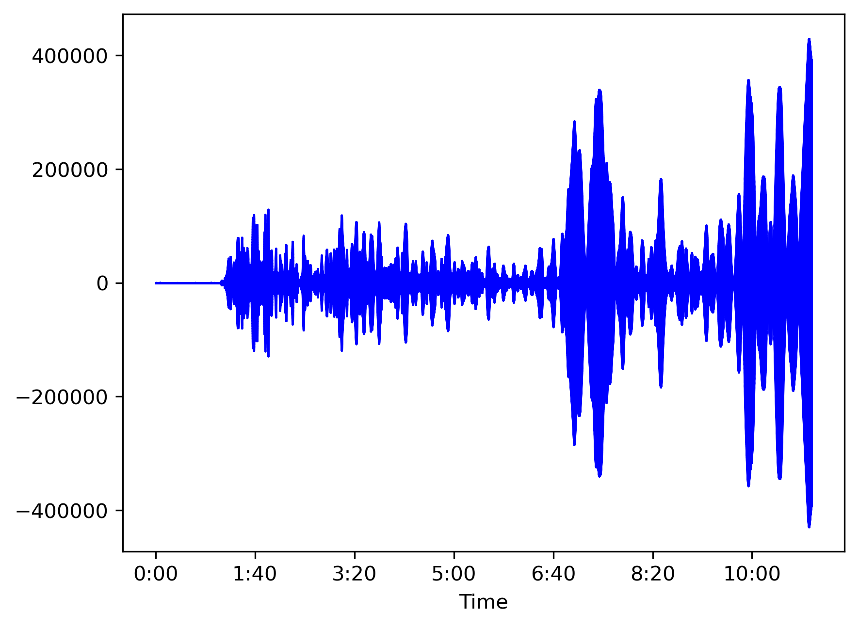
Let us select an event: 2021-07-29 Mww8.2 Alaska Peninsula, and a station to look at the waveforms: PFO: Pinon Flat, California, USA. The data is raw and downloaded from IRIS.
Plot waveforms
from obspy import read
import librosa
import librosa.display
import matplotlib.pyplot as plt
import numpy as np

dataFile = '2021-07-29-mww82-alaska-peninsula-2.miniseed'

st0 = read(dataFile)
st = st0.select(channel='BHZ', location='00')
print(st)

# play with hop_length and nfft values
hop_length = 128
n_fft = 256
cmap = 'jet'
bins_per_octave = 12
auto_aspect = False
y_axis = "linear"  # linear or log
fmin = None
fmax = 5.0

data = st[0].data.astype('float32')
sr = int(st[0].stats.sampling_rate)
max_points = int(st[0].stats.npts)
offset = 0

# Waveplot
fig, ax = plt.subplots()
librosa.display.waveshow(data, sr=sr, max_points=max_points,
                         x_axis='time', offset=offset, color='b', ax=ax)
plt.savefig('waveplot.png', bbox_inches='tight', dpi=300)
plt.close()
A note on waveshow. This code already uses librosa.display.waveshow, which replaced the old waveplot (removed in librosa 0.9). If you’re following an older tutorial that calls librosa.display.waveplot(...), swap it for waveshow on any current librosa (the latest is 0.11). Since librosa 0.9, most functions also expect keyword arguments rather than positional ones — which the snippets here already do.
Plot spectrogram
# Librosa spectrogram
D = librosa.amplitude_to_db(
    np.abs(librosa.stft(data, hop_length=hop_length, n_fft=n_fft)), ref=np.max)


fig, ax = plt.subplots()

img = librosa.display.specshow(D, y_axis=y_axis, sr=sr,
                               hop_length=hop_length, x_axis='time', ax=ax, cmap=cmap, bins_per_octave=bins_per_octave,
                               auto_aspect=auto_aspect)

if fmin is not None:
    fmin0 = fmin
else:
    fmin0 = 0

if fmax is not None:
    fmax0 = fmax
else:
    fmax0 = sr/2

ax.set_ylim([fmin, fmax])
fig.colorbar(img, ax=ax, format="%+2.f dB")
plt.savefig('spectrogram.png', bbox_inches='tight', dpi=300)
plt.close()
That one dense line mirrors the diagram exactly: librosa.stft(...) computes the complex STFT with your n_fft/hop_length, np.abs(...) takes the magnitude, and librosa.amplitude_to_db(..., ref=np.max) rescales to decibels relative to the loudest bin. specshow then draws the frequency-by-time array, and set_ylim crops to the band you care about (here fmax = 5.0 Hz, since seismic energy is low-frequency).
Quick check: You increase n_fft (a longer STFT window) while keeping everything else fixed. What happens?
Recap
- Spectrogram = STFT magnitude in dB. Slide a window, FFT each chunk, take the magnitude, convert to decibels, and display.
- Two knobs, one trade-off.
n_fftsets frequency resolution;hop_lengthsets time resolution — you can’t sharpen both at once. - librosa is built for speed. Designed for large audio corpora, it computes the STFT for long series (seismic included) in seconds where naive methods stall.
- Use the current API.
waveshow(notwaveplot) andamplitude_to_db/power_to_db(notlogamplitude); pass parameters by keyword.
Where to go next
- librosa
stftdocs: librosa.org/doc/latest/generated/librosa.stft.html - librosa
display.specshowdocs: librosa.org/doc/latest/generated/librosa.display.specshow.html - Earlier ObsPy spectrogram approach: Concatenating daily seismic traces and plotting a spectrogram
References
McFee, B., Raffel, C., Liang, D., Ellis, D. P. W., McVicar, M., Battenberg, E., & Nieto, O. (2015). librosa: Audio and music signal analysis in Python. In K. Huff & J. Bergstra (Eds.), Proceedings of the 14th Python in Science Conference (pp. 18–24). https://doi.org/10.25080/majora-7b98e3ed-003
Schörkhuber, C., & Klapuri, A. (2010). Constant-Q transform toolbox for music processing. Proceedings of the 7th Sound and Music Computing Conference. https://doi.org/10.5281/zenodo.849741
Resources
- librosa: Audio and Music Signal Analysis in Python — Brian McFee — YouTube video.
Found this article useful?
Loading likes…
Disclaimer of liability
The information provided by the Earth Inversion is made available for educational purposes only.
Whilst we endeavor to keep the information up-to-date and correct. Earth Inversion makes no representations or warranties of any kind, express or implied about the completeness, accuracy, reliability, suitability or availability with respect to the website or the information, products, services or related graphics content on the website for any purpose.
UNDER NO CIRCUMSTANCE SHALL WE HAVE ANY LIABILITY TO YOU FOR ANY LOSS OR DAMAGE OF ANY KIND INCURRED AS A RESULT OF THE USE OF THE SITE OR RELIANCE ON ANY INFORMATION PROVIDED ON THE SITE. ANY RELIANCE YOU PLACED ON SUCH MATERIAL IS THEREFORE STRICTLY AT YOUR OWN RISK.
Leave a comment