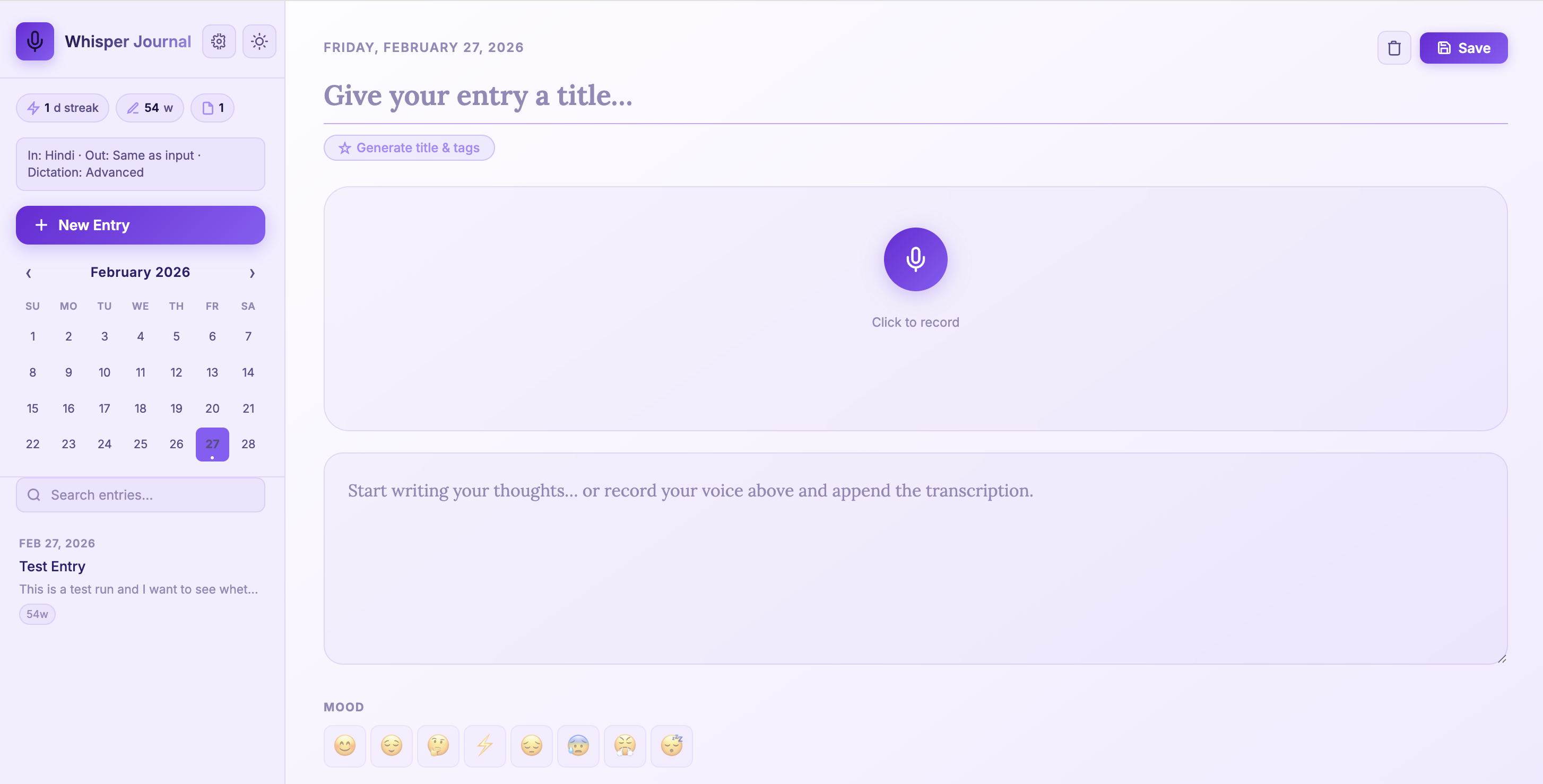
Build a Multilingual Local Voice Journal App with FastAPI and Whisper (Beginner Guide)
A beginner-friendly walkthrough to build and run Whisper Journal with multilingual dictation, local Whisper...

Earth Inversion
Technical writing on geophysical pipelines, scalable data analysis, and reproducible research engineering.
Peer-reviewed work in seismology, structural health monitoring, and large-scale inversion.
End-to-end workflows for high-volume scientific data: ingestion, QC, feature extraction, and modeling.
Cloud and web platforms for real-time sensing, visualization, and operational analytics.
A beginner-friendly walkthrough to build and run Whisper Journal with multilingual dictation, local Whisper...
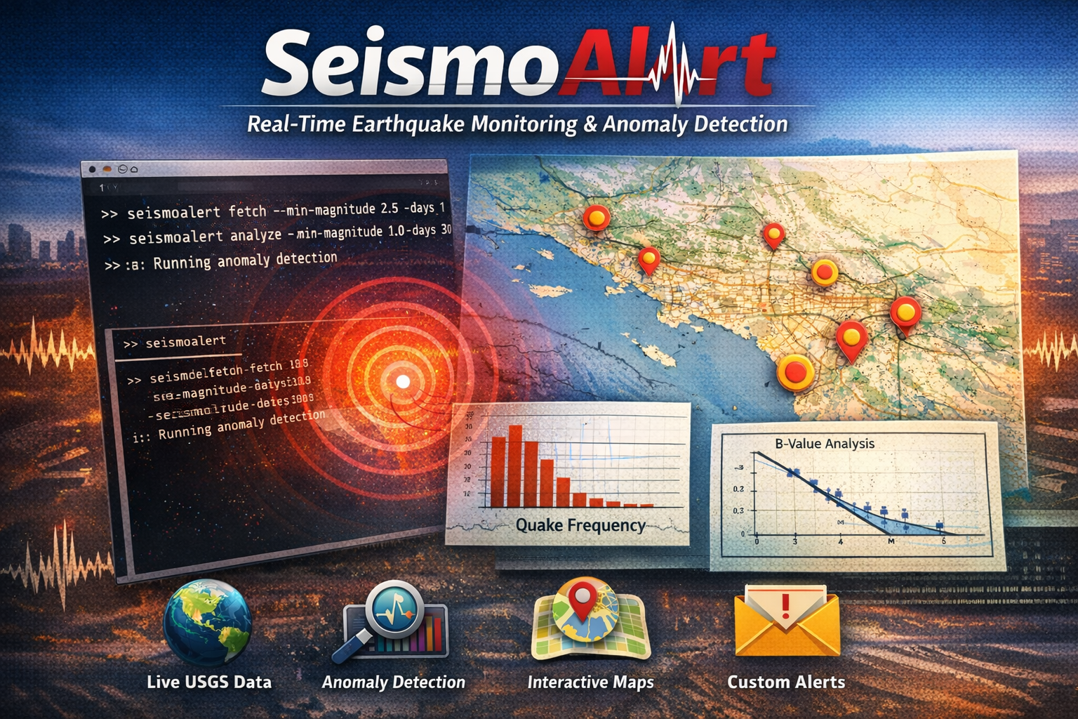
I built SeismoAlert to fetch USGS earthquake data, run statistical analysis, detect anomalies, and generate...
Recent technical articles on seismic analytics, scientific computing, numerical modeling, and production data workflows.
A practical, beginner-friendly walkthrough of a complete FastAPI DevOps workflow: clean code, layered testing, CI with Jenkins and GitHub Actions, and runtim...
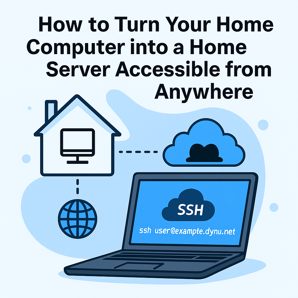
Turn your everyday computer into a home server you can access from anywhere using Dynamic DNS, a simple update script, and secure SSH access.
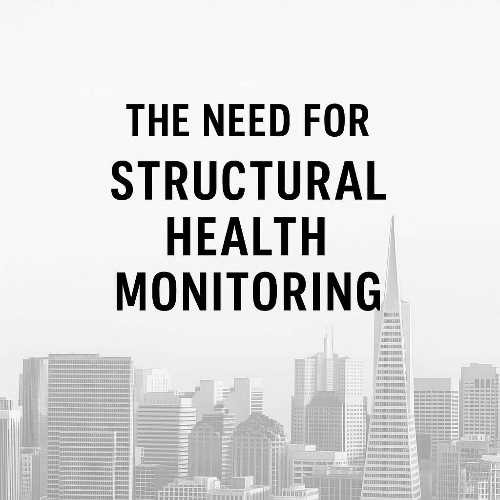
The San Francisco Bay Area combines high seismic hazard, dense urban exposure, and aging infrastructure. Structural Health Monitoring can improve post-earthq...
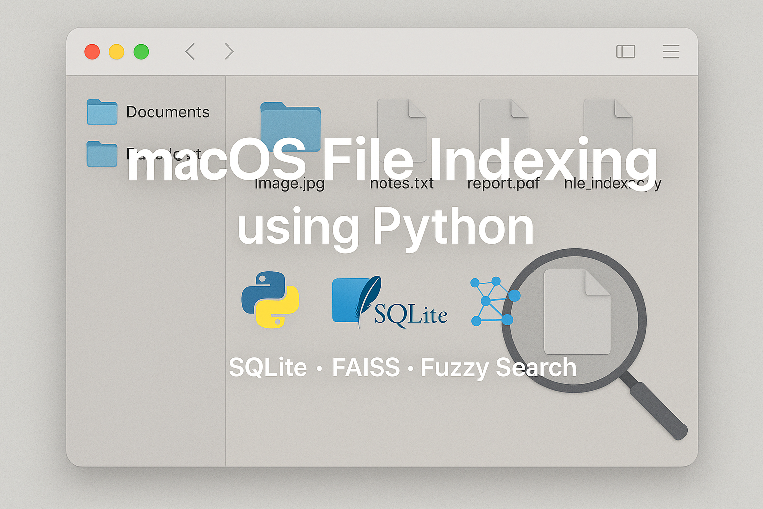
A Python-based solution for indexing and searching files on a macOS system using SQLite, FAISS, and semantic search.
Cloud computing is transforming geophysical and seismological research by enabling scalable processing, faster collaboration, and reproducible workflows for ...
A practical introduction to Docker for geophysics students, including images, containers, volumes, and a simple workflow for reproducible seismic data analys...
Learn how to set up Databricks, create your first Spark cluster, upload data, and run PySpark notebooks for scalable big data analysis.
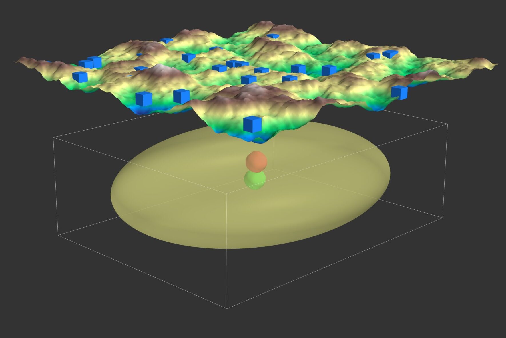
Discover how Genetic Algorithms can be applied to solve the earthquake location problem in seismology. This post walks through generating synthetic seismic d...
Learn how to seamlessly sync your Zotero files across devices using WebDAV with Koofr and Google Drive. This step-by-step guide ensures your research materia...
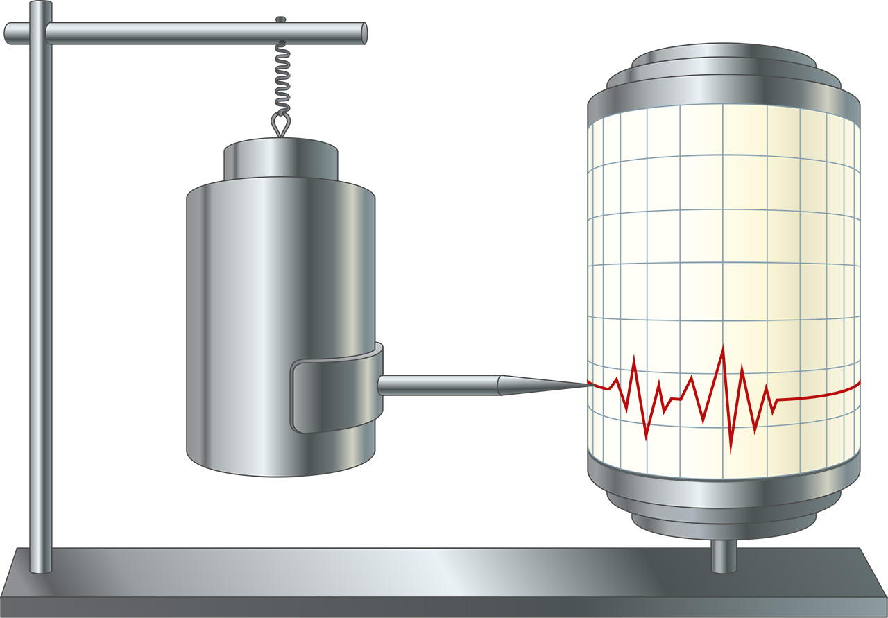
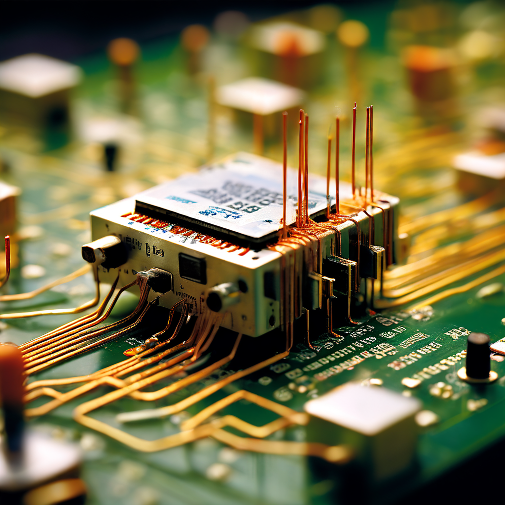
While MEMS accelerometers offer advantages in cost, size, and deployment flexibility compared to traditional broadband seismometers, they face limitations in...
While MEMS accelerometers offer advantages in cost, size, and deployment flexibility compared to traditional broadband seismometers, they face limitations in...
Scientists have detected low-frequency gravitational waves permeating the entire universe, opening a new window into cosmic phenomena. This groundbreaking di...
A practical, beginner-friendly walkthrough of a complete FastAPI DevOps workflow: clean code, layered testing, CI with Jenkins and GitHub Actions, and runtim...
Turn your everyday computer into a home server you can access from anywhere using Dynamic DNS, a simple update script, and secure SSH access.
The San Francisco Bay Area combines high seismic hazard, dense urban exposure, and aging infrastructure. Structural Health Monitoring can improve post-earthq...
A Python-based solution for indexing and searching files on a macOS system using SQLite, FAISS, and semantic search.
Cloud computing is transforming geophysical and seismological research by enabling scalable processing, faster collaboration, and reproducible workflows for ...
A practical introduction to Docker for geophysics students, including images, containers, volumes, and a simple workflow for reproducible seismic data analys...
Learn how to set up Databricks, create your first Spark cluster, upload data, and run PySpark notebooks for scalable big data analysis.
Discover how Genetic Algorithms can be applied to solve the earthquake location problem in seismology. This post walks through generating synthetic seismic d...
Learn how to seamlessly sync your Zotero files across devices using WebDAV with Koofr and Google Drive. This step-by-step guide ensures your research materia...
While MEMS accelerometers offer advantages in cost, size, and deployment flexibility compared to traditional broadband seismometers, they face limitations in...
While MEMS accelerometers offer advantages in cost, size, and deployment flexibility compared to traditional broadband seismometers, they face limitations in...
Scientists have detected low-frequency gravitational waves permeating the entire universe, opening a new window into cosmic phenomena. This groundbreaking di...