Introduction to Numpy for scientific computing
Loading likes…
Numpy is a numerical processing library in Python that is capable of efficiently handling large datasets. It is the building block of many libraries such as Pandas, SciPy, Scikit-learn, etc. It is incredibly fast given its bindings to C libraries.
In this post, we will focus only on the basics as the capabilities and possibilities with Numpy are immense and it is not possible to cover everything in one post. For quickly jumping between different topics, use the “contents” that has been linked to the topics by hyperlinks.
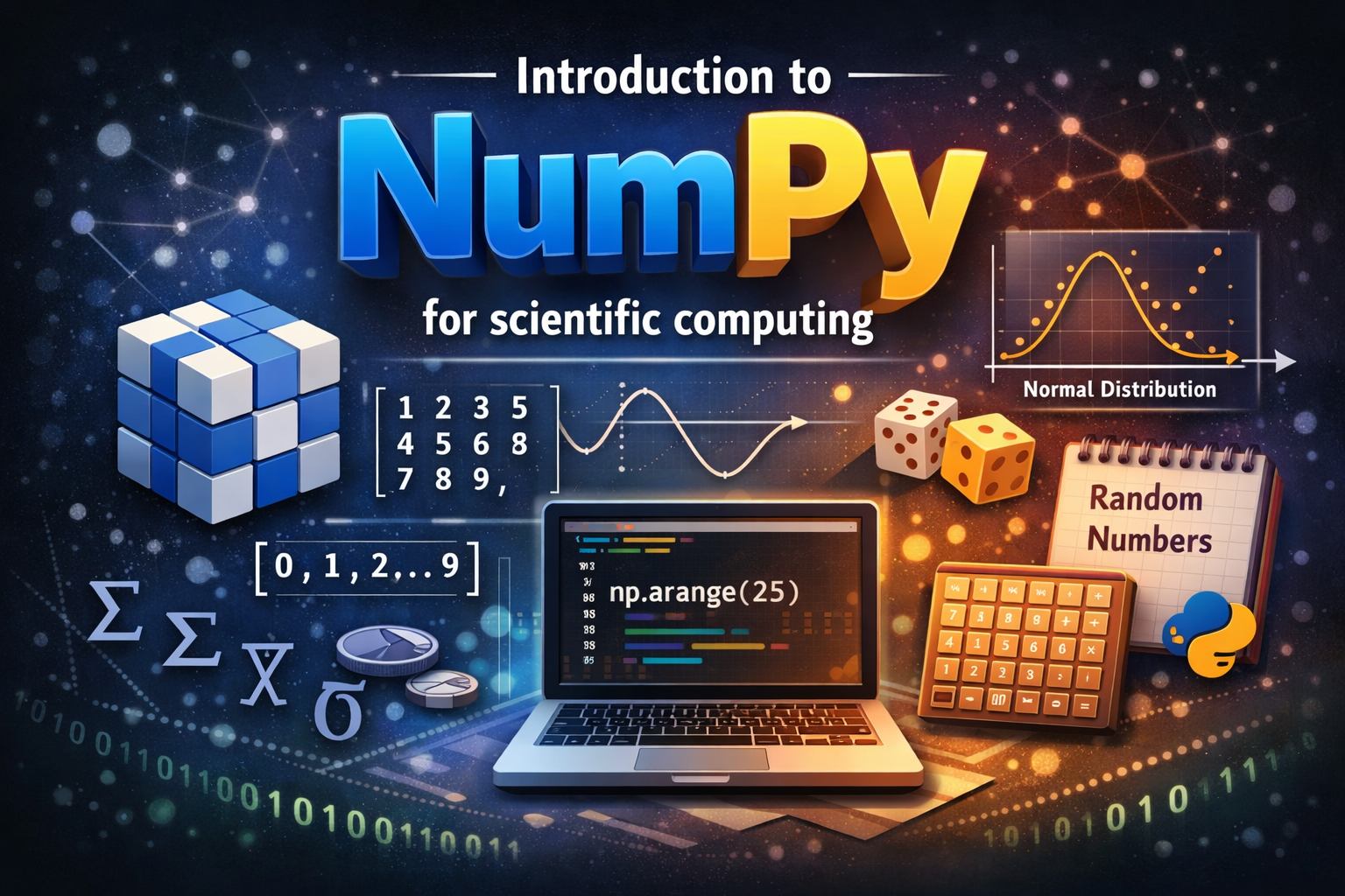
Key idea — one typed array + whole-array operations = speed. A NumPy ndarray stores its numbers in a single contiguous block of one dtype, described by a shape. Because of that, you operate on the whole array at once — a + b, np.sqrt(arr), arr[arr>5] — with no Python loop; the work happens in fast C under the hood. That’s vectorization, and it’s why NumPy underpins Pandas, SciPy, and scikit-learn. One gotcha to learn early: a slice is a view (it shares memory with the original), so use .copy() when you need an independent array.
a + b over the whole array in one C-level operation instead of a Python loop.Create numpy arrays
1-D array
import numpy as np #we give an alias to numpy
mylist = [1, 2, 3] #create a list
myarray = np.array(mylist) #convert list to array
Higher dimensional arrays (or matrix)
my_matrix = [[1,2,3],[4,5,6],[7,8,9]]
my_np_matrix = np.array(my_matrix)
print(my_np_matrix)
This returns (=>):
[[1 2 3]
 [4 5 6]
 [7 8 9]]
Methods and attributes in numpy
We can access the methods or attributes in numpy by using the “.”.
print(my_np_matrix.shape)
=>
(3, 3)
print(my_np_matrix.mean())
=>
5.0
reshape
arr = np.arange(25)
print(arr)
reshaped_arr = arr.reshape(5,5)
print(reshaped_arr)
We use the same data and shape it into new dimension =>
[ 0  1  2  3  4  5  6  7  8  9 10 11 12 13 14 15 16 17 18 19 20 21 22 23
 24]
[[ 0  1  2  3  4]
 [ 5  6  7  8  9]
 [10 11 12 13 14]
 [15 16 17 18 19]
 [20 21 22 23 24]]
Also, keep in mind that we cannot use any shape we want here. Since, the original dataset had only 25 elements, we can reshape it into 5 x 5, 1 x 25, 25 x 1, etc.
minimum, maximum and its indices
ranarr = np.random.randint(34, 68, 10)
print(ranarr)
print(ranarr.max())
print(ranarr.argmax())
print(ranarr.min())
print(ranarr.argmin())
=>
[40 37 36 62 44 54 54 67 54 63]
67
7
36
2
datatype with dtype
print(ranarr.dtype)
=>
int64
Built-in Methods in numpy
arange
a = np.arange(0,10)
print(a)
b = np.arange(0,11,2)
print(b)
=>
[0 1 2 3 4 5 6 7 8 9]
[ 0  2  4  6  8 10]
zeros and ones
twod_zeros = np.zeros((5,5))
print(twod_zeros)

twod_ones = np.ones((3,3)) #make two dimensional array of ones
print(twod_ones)
=>
[[0. 0. 0. 0. 0.]
 [0. 0. 0. 0. 0.]
 [0. 0. 0. 0. 0.]
 [0. 0. 0. 0. 0.]
 [0. 0. 0. 0. 0.]]

[[1. 1. 1.]
[1. 1. 1.]
[1. 1. 1.]]
twod_ones_new = twod_ones * 100
print(twod_ones_new)
=>
[[100. 100. 100.]
 [100. 100. 100.]
 [100. 100. 100.]]
linspace for evenly spaced numbers
Z = np.linspace(0,5,20)
print(Z)
This gives 20 linearly spaced numbers between 0 and 5.
=>
[0.         0.26315789 0.52631579 0.78947368 1.05263158 1.31578947
 1.57894737 1.84210526 2.10526316 2.36842105 2.63157895 2.89473684
 3.15789474 3.42105263 3.68421053 3.94736842 4.21052632 4.47368421
 4.73684211 5.        ]
identity matrix with eye
I = np.eye(4)
print(I)
=>
[[1. 0. 0. 0.]
 [0. 1. 0. 0.]
 [0. 0. 1. 0.]
 [0. 0. 0. 1.]]
Random numbers in Numpy
From uniform distribution
myrand = np.random.rand(2)
print(myrand)
This creates an array of the specified shape and populates it with random samples from a uniform distribution over [0, 1).
=>
[0.8300824 0.93838919]
myrand2 = np.random.rand(5,5)
print(myrand2)
=>
[[0.56931238 0.0130365  0.49126232 0.87114911 0.76042729]
 [0.09251311 0.82855503 0.63039485 0.97381338 0.01540617]
 [0.97649667 0.30297094 0.26201115 0.64828968 0.44611475]
 [0.71639265 0.93906588 0.31467679 0.82751456 0.13620669]
 [0.04310447 0.22531851 0.69068734 0.43045271 0.44482673]]
From standard normal distribution
mynrand = np.random.randn(2)
print(mynrand)
=>
[-0.40174504 0.00292135]
Random integers
myrandint = np.random.randint(1,100)
print(myrandint)
print(np.random.randint(1,100,10))
=>
82
[94 80 31 18 62 69 26 71 64 93]
Set the random state with seed
np.random.seed(12)
print(np.random.rand(4))
You should get the same exact output as me if you use the same seed as above. =>
[0.15416284 0.7400497 0.26331502 0.53373939]
Numpy Indexing
Let us first create a simple array to start with:
arr = np.arange(0,11)
print(arr)
=>
[ 0 1 2 3 4 5 6 7 8 9 10]
To get a value at an index or in a range of indexes:
print(arr[8])
#Get values in a range
print(arr[0:5])
=>
8
[0 1 2 3 4]
Broadcating values at a range of indexes
Unlike Python lists, with NumPy arrays, one can broadcast a single value across a larger set of values.
arr[0:5]=120

print(arr)
print(arr **2)
=>
[120 120 120 120 120   5   6   7   8   9  10]
[14400 14400 14400 14400 14400    25    36    49    64    81   100]
We can also use this design to extract the slice of an array:
print(arr)
#Important notes on Slices
slice_of_arr = arr[0:6]

#Show slice
print(slice_of_arr)
=>
[120 120 120 120 120   5   6   7   8   9  10]
[120 120 120 120 120   5]
Another good point about slicing in Numpy is that the data is not being copied but still pointing to the original array. This avoids memory problems.
arr = np.arange(0,11)
print(arr)

#Change Slice
slice_of_arr = arr[0:6]
slice_of_arr[:]=99

#Show Slice again
print(slice_of_arr)
print(arr)
=>
[ 0  1  2  3  4  5  6  7  8  9 10]
[99 99 99 99 99 99]
[99 99 99 99 99 99  6  7  8  9 10]
We can avoid this using the copy method.
arr = np.arange(0,11)
print(arr)


#To get a copy, need to be explicit
arr_copy = arr.copy()

print(arr_copy)

#Change Slice
slice_of_arr = arr_copy[0:6]
slice_of_arr[:]=99

#Show Slice again
print(slice_of_arr)
print(arr)
print(arr_copy)
=>
[ 0  1  2  3  4  5  6  7  8  9 10]
[ 0  1  2  3  4  5  6  7  8  9 10]
[99 99 99 99 99 99]
[ 0  1  2  3  4  5  6  7  8  9 10]
[99 99 99 99 99 99  6  7  8  9 10]
Quick check: You take s = arr[0:6] and then do s[:] = 99. Why does the original arr change too?
Indexing a 2D array
arr_2d = np.array(([5,10,15],[20,25,30],[35,40,45]))

#Show
print(arr_2d)
=>
[[ 5 10 15]
 [20 25 30]
 [35 40 45]]
# Getting individual element value
print(arr_2d[1][0]) # Format is arr_2d[row][col] or arr_2d[row,col]
# or
print(arr_2d[1,0])

print(arr_2d[:2,1:])

print(arr_2d[:2,1:]) #(2,2) from top right corner
=>
20
20
[[10 15]
 [25 30]]
Conditional Selection
arr = np.arange(1,11)
print(arr)
print(arr > 5)
=>
[ 1  2  3  4  5  6  7  8  9 10]
[False False False False False  True  True  True  True  True]
print(arr[arr>5])
print(arr[(arr>5) & (arr<9)])
=>
[ 6  7  8  9 10]
[6 7 8]
Numpy Operations
arr = np.arange(0,10)
print(arr)
=>
[0 1 2 3 4 5 6 7 8 9]
Simple arithmetics
print(arr + arr)
print(arr * arr)
print(arr**3)
=>
[ 0  2  4  6  8 10 12 14 16 18]
[ 0  1  4  9 16 25 36 49 64 81]
[  0   1   8  27  64 125 216 343 512 729]
Universal array functions
Check the numpy documentation for the list of all the universal functions: ufuncs in numpy
# Taking Square Roots
print(np.sqrt(arr))

# Trigonometric Functions like sine
print(np.sin(arr))
=>
[0.         1.         1.41421356 1.73205081 2.         2.23606798
 2.44948974 2.64575131 2.82842712 3.        ]
[ 0.          0.84147098  0.90929743  0.14112001 -0.7568025  -0.95892427
-0.2794155   0.6569866   0.98935825  0.41211849]
Dealing with different axes
In numpy array, axis 0 (zero) is the vertical axis (rows), and axis 1 is the horizonal axis (columns).
arr_2d = np.array([[1,2,3,4],[5,6,7,8],[9,10,11,12]])
print(arr_2d)
=>
[[ 1  2  3  4]
 [ 5  6  7  8]
 [ 9 10 11 12]]
print(arr_2d.sum(axis=0)) #returns the sum across rows
print(arr_2d.sum(axis=1)) #returns the sum across columns
=>
[15 18 21 24]
[10 26 42]
Next, in the series of Python tutorials is “Pandas”.
Modern-NumPy note. Everything above works unchanged on current NumPy (2.x). Two habits worth adopting: (1) for random numbers, the recommended API is now a Generator — rng = np.random.default_rng(seed); rng.random(4) — rather than the legacy global np.random.seed/np.random.rand used here (both still work). (2) Avoid np.matrix (long deprecated); use plain 2-D arrays as this post does.
Recap
ndarray= shape + dtype + one contiguous buffer. That layout is what makes operations fast.- Vectorize, don’t loop.
a + b,np.sqrt(arr),arr[arr>5]act on the whole array in C — no Python loop. - Views vs copies. A slice shares memory with the original; call
.copy()for an independent array. - Axes matter.
axis=0reduces down columns (across rows),axis=1reduces across columns. - Everything builds on this. Pandas, SciPy, scikit-learn, and PyTorch all sit on top of the NumPy array.
Where to go next
- Next in the series — Pandas: How to start using Pandas for Earth data analysis
- NumPy arrays with a deep-learning twist — PyTorch tensors: Getting familiar with PyTorch data structures
- Official NumPy user guide: numpy.org/doc/stable/user
References
- Photo by Karl Magnuson on Unsplash
Found this article useful?
Loading likes…
Disclaimer of liability
The information provided by the Earth Inversion is made available for educational purposes only.
Whilst we endeavor to keep the information up-to-date and correct. Earth Inversion makes no representations or warranties of any kind, express or implied about the completeness, accuracy, reliability, suitability or availability with respect to the website or the information, products, services or related graphics content on the website for any purpose.
UNDER NO CIRCUMSTANCE SHALL WE HAVE ANY LIABILITY TO YOU FOR ANY LOSS OR DAMAGE OF ANY KIND INCURRED AS A RESULT OF THE USE OF THE SITE OR RELIANCE ON ANY INFORMATION PROVIDED ON THE SITE. ANY RELIANCE YOU PLACED ON SUCH MATERIAL IS THEREFORE STRICTLY AT YOUR OWN RISK.
Leave a comment