Analyzing MiniSEED seismic data in MATLAB (codes included)

I have a MiniSEED (or mseed) file and I want to analyze it in MATLAB. But unfortunately, MATLAB can’t read mseed file. So, let us figure out how can we read and analyze it using MATLAB.

What is MiniSEED format?

IRIS uses SEED as a data format intended primarily for the archival and exchange of seismological time series data and related metadata. MiniSEED is a stripped down version of SEED containing only waveform data. There is no station and channel metadata included. See here for more.

Utitlity program to convert MiniSEED into MAT format

I wrote a utility program that uses the Obspy library in Python to convert the mseed file to mat format. You can download the utility from here.

usage: convert_mseed_mat.py [-h] -inp INPUT_MSEED [-out OUTPUT_MAT]

Python utility program to convert mseed file to mat (by Utpal Kumar, IESAS, 2021/04)

optional arguments:
  -h, --help            show this help message and exit
  -inp INPUT_MSEED, --input_mseed INPUT_MSEED
                        input mseed file, e.g. example_2020-05-01_IN.RAGD..BHZ.mseed
  -out OUTPUT_MAT, --output_mat OUTPUT_MAT
                        output mat file name, e.g. example_2020-05-01_IN.RAGD..BHZ.mat

Let us see an example:

python convert_mseed_mat.py -inp example_2020-05-01_IN.RAGD..BHZ.mseed

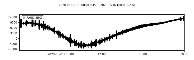
Output data structure

• stats contains all the meta data information corresponding to each trace and
• data contain the time series data

mat_file.mat -> stats, data
stats -> stats_0, stats_1, ...
data -> data_0, data_1, ...

Read mat file in MATLAB

Now, let us read the mat file containing the seismic time series data. We start by the usual initializing the MATLAB and reading the file name.

clear; close all; clc;

wdir='.\';

fileloc0=[wdir,'example_2020-05-01_IN.RAGD..BHZ'];
fileloc_ext = '.mat';
fileloc = [fileloc0 fileloc_ext];

Plot time series

We now check if the mat file exists, and the read the meta data stored in stats_0. We get the sampling_rate, delta, starttime, endtime. For plotting, we create the datetime_array.

if exist(fileloc,'file')
    disp(['File exists ', fileloc]);
    load(fileloc);
    
    all_stats = fieldnames(stats);
    all_data = fieldnames(data);
    
        
%     for id=1:length(fieldnames(data))
    for id=1
        stats_0 = stats.(all_stats{id});
        data_0 = data.(all_data{id});

        sampling_rate = getfield(stats_0,'sampling_rate');
        delta = getfield(stats_0,'delta');
        starttime = getfield(stats_0,'starttime');
        endtime = getfield(stats_0,'endtime');
        t1 = datetime(starttime,'InputFormat',"yyyy-MM-dd'T'HH:mm:ss.SSS'Z'");
        t2 = datetime(endtime,'InputFormat',"yyyy-MM-dd'T'HH:mm:ss.SSS'Z'");
        datetime_array = t1:seconds(delta):t2;

        %% plot time series
        fig = figure('Renderer', 'painters', 'Position', [100 100 1000 400], 'color','w');
        plot(t1:seconds(delta):t2, data_0, 'k-')
        title([getfield(stats_0,'network'),'-', getfield(stats_0,'station'), '-', getfield(stats_0,'channel')])
        axis tight;
        print(fig,['docs/',fileloc0, '_ts', num2str(id),'.jpg'],'-djpeg')

%         close all;
    end
end

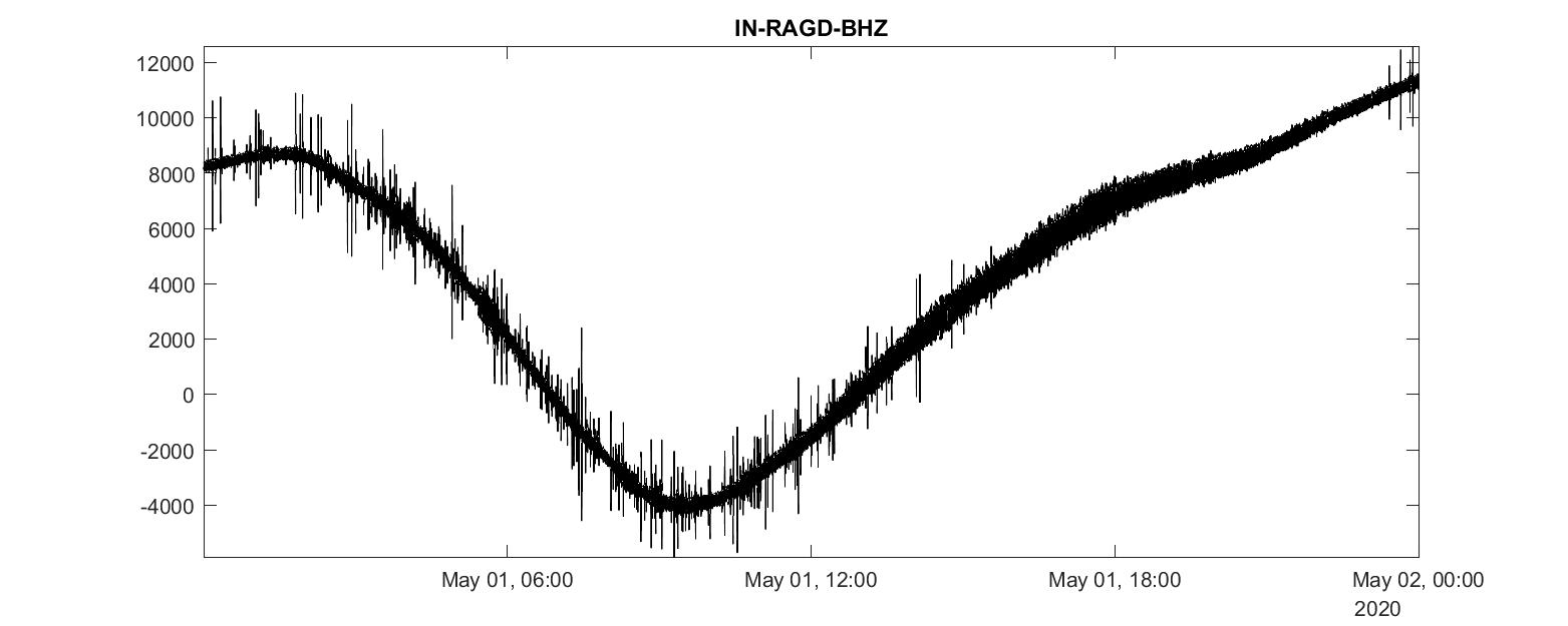
Plot spectrogram

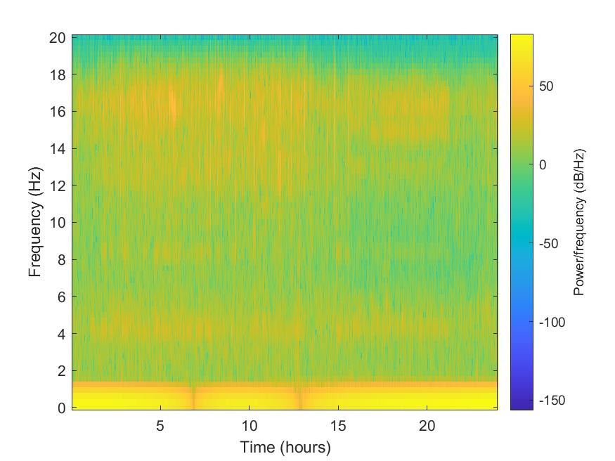
We used the spectrogram function from MATLAB to plot the spectrogram (can be improved further). We divide the signal into sections of length 128, windowed with a Kaiser window with shape parameter $\beta = 18$ and specify 120 samples of overlap between adjoining sections. We evaluate the spectrum at 65 frequencies and $(\text{length}(x)-120)/(128-120)=235$ time bins.

if exist(fileloc,'file')
    disp(['File exists ', fileloc]);
    load(fileloc);
    
    all_stats = fieldnames(stats);
    all_data = fieldnames(data);
    
        
%     for id=1:length(fieldnames(data))
    for id=1
        stats_0 = stats.(all_stats{id});
        data_0 = data.(all_data{id});

        sampling_rate = getfield(stats_0,'sampling_rate');

        fig2 = figure('Renderer', 'painters', 'Position', [100 100 1000 400], 'color','w');
        data_0_double = double(data_0);
        
        spectrogram(data_0_double,kaiser(128,18),120,128,sampling_rate,'yaxis')

        %% if you want to normalize the frequency axis in range 0 to 1
%         yticks([0 sampling_rate/4 sampling_rate/2])
%         yticklabels({'0','0.5','1'})
%         ylabel('Normalized Frequency');
        
        title([getfield(stats_0,'network'),'-', getfield(stats_0,'station'), '-', getfield(stats_0,'channel')])
        print(fig2,['docs/',fileloc0, '_spectrogram', num2str(id),'.jpg'],'-djpeg')
%         close all;
    end
end

Conclusions

Converting Miniseed into mat format allows us to easily read the seismic time series data in MATLAB. Once we load the data in MATLAB, we can make use of all the avilable MATLAB commands and tools.

Recap

• Python is the bridge. ObsPy reads MiniSEED and scipy.io.savemat writes a .mat — the format MATLAB opens natively.
• Keep metadata + data. The converter stores stats (headers) and data (samples) so you can rebuild an accurate time axis in MATLAB.
• Then it’s plain MATLAB. load the .mat, read fields from stats_0, build a datetime array, and plot / spectrogram as usual.
• Spectrogram knobs. The spectrogram(x, kaiser(128,18), 120, 128, fs, 'yaxis') call sets window, overlap, FFT length and sampling rate — tune them for the time–frequency trade-off.

Where to go next

• The converter (GitHub): github.com/earthinversion/convert-mseed2mat
• MATLAB spectrogram docs: mathworks.com/help/signal/ref/spectrogram.html
• Denoise the loaded data — MATLAB wavelet analysis: How effective is signal denoising using MATLAB wavelet analysis