Numerical optimization based on the L-BFGS method

In this post, we will inspect the Limited-memory Broyden, Fletcher, Goldfarb, and Shanno (L-BFGS) optimization method using one minimization example for the Rosenbrock function. Further, we will compare the performance of the L-BFGS method with the gradient-descent method. The L-BFGS approach along with several other numerical optimization routines, are at the core of machine learning.

Introduction

Optimization problems aim at finding the minima or maxima of a given objective function. There are two deterministic approaches to optimization problems - first-order derivative (such as gradient descent, steepest descent) and second-order derivative methods (such as Newton’s method). The first-order derivative methods rely on following the derivative (or gradient) downhill/uphill to find the function’s maxima/maxima (optimal solution). The second-order derivative methods that are based on the derivative of the derivative (Hessian, a matrix containing the second derivatives) can more efficiently estimate the minima of the objective functions. This is because second-order derivatives give us the direction towards the optimal solution and the required step size.

The L-BFGS method is a type of second-order optimization algorithm and belongs to a class of Quasi-Newton methods. It approximates the second derivative for the problems where it cannot be directly calculated. Newton’s method uses the Hessian matrix (as it is a second-order derivative method). However, it has a limitation as it requires the calculation of the inverse of the Hessian that can be computationally intensive. The Quasi-Newton method approximates the inverse of the Hessian using the gradient and hence can be computationally feasible.

The BFGS method (the L-BFGS is an extension of BFGS) updates the calculation of the Hessian matrix at each iteration rather than recalculating it. However, the size of the Hessian and its inverse is dependent on the number of input parameters to the objective function. Hence, for a large problem, the size of the Hessian can be an issue to deal with. The L-BFGS solves this by assuming a simplification of the inverse of the Hessian in the previous iteration. Unlike BFGS, which is based on full history of the gradients, L-BFGS is based on the most recent n gradients (typically 5-20, a much smaller storage requirement).

Newton’s method

Let us mathematically see how we solve the Newton’s method:

Using Taylor’s expansion, we can write the twice-differentiable function, $f(t)$ as

where $\Delta f(t)$ and $\Delta^2 f(t)$ are the gradient and Hessian of $f(t)$ at the point $x$. This is assuming $\Delta t$ is very small.

where, $g_n$ and $\mathbf{H}_n$ are the gradient and Hessian of $f(t)$ at $t_n$. In order to obtain the $\Delta t$ the $f(t)$, we differentiate the above function by $\Delta t$.

To obtain the minima/maxima, we assume $\frac{\partial h_n(\Delta t)}{\partial \Delta t} = 0$ and $\mathbf{H}_n$ to be positive definite. This gives

\(\Delta t = - \mathbf{H}_n^{-1} g_n\) This gives the step size to move in the direction of optimal point.

L-BFGS implementation for the Rosenbrock function

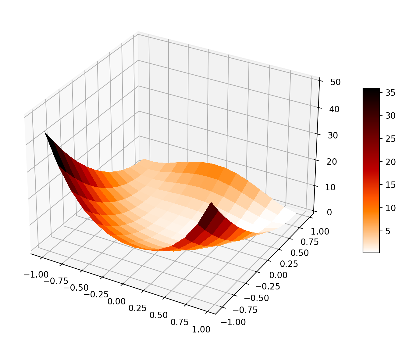
Rosenbrock function is a non-convex function used as a performance test for optimization algorithms.

# l-bfgs-b algorithm local optimization of a convex function
from scipy.optimize import minimize
from scipy.optimize import rosen, rosen_der
import numpy as np
from matplotlib import cm
import matplotlib.pyplot as plt
import time
np.random.seed(122)


def plot_objective(objective):
    # Initialize figure 
    figRos = plt.figure(figsize=(12, 7))
    axRos = plt.subplot(111, projection='3d')

    # Evaluate function
    X = np.arange(-1, 1, 0.15)
    Y = np.arange(-1, 1, 0.15)
    X, Y = np.meshgrid(X, Y)
    XX = (X,Y)
    Z = objective(XX)

    # Plot the surface
    surf = axRos.plot_surface(X, Y, Z, cmap=cm.gist_heat_r,
                        linewidth=0, antialiased=False)
    axRos.set_zlim(0, 50)
    figRos.colorbar(surf, shrink=0.5, aspect=10)
    plt.savefig('objective_function.png',bbox_inches='tight', dpi=200)
    plt.close()


## Rosenbrock function
# objective function
b = 10
def objective(x):
    f = (x[0]-1)**2 + b*(x[1]-x[0]**2)**2
    return f


plot_objective(objective)

# derivative of the objective function
def derivative(x):
    df = np.array([2*(x[0]-1) - 4*b*(x[1] - x[0]**2)*x[0], \
                         2*b*(x[1]-x[0]**2)])
    return df


starttime = time.perf_counter()
# define range for input
r_min, r_max = -1.0, 1.0

# define the starting point as a random sample from the domain
pt = r_min + np.random.rand(2) * (r_max - r_min)
print('initial input pt: ', pt)

# perform the l-bfgs-b algorithm search
result = minimize(objective, pt, method='L-BFGS-B', jac=derivative)
print(f"Total time taken for the minimization: {time.perf_counter()-starttime:.4f}s")
# summarize the result
print('Status : %s' % result['message'])
print('Total Evaluations: %d' % result['nfev'])


# evaluate solution
solution = result['x']
evaluation = objective(solution)
print('Solution: f(%s) = %.5f' % (solution, evaluation))

This gives

$ python lbfgs_algo.py 
initial input pt:  [-0.68601632  0.40442008]
Total time taken for the minimization: 0.0046s
Status : CONVERGENCE: NORM_OF_PROJECTED_GRADIENT_<=_PGTOL
Total Evaluations: 24
Solution: f([1.0000006  1.00000115]) = 0.00000

It took 0.0046s for the method to converge to the minima in 24 iterations.

Gradient descent method

import numpy as np
import time
starttime = time.perf_counter()

# define range for input
r_min, r_max = -1.0, 1.0

# define the starting point as a random sample from the domain
cur_x = r_min + np.random.rand(2) * (r_max - r_min)

rate = 0.01 # Learning rate
precision = 0.000001 #This tells us when to stop the algorithm
previous_step_size = 1 #
max_iters = 10000 # maximum number of iterations
iters = 0 #iteration counter


## Rosenbrock function
# objective function
b = 10
def objective(x):
    f = (x[0]-1)**2 + b*(x[1]-x[0]**2)**2
    return f


# derivative of the objective function
def derivative(x):
    df = np.array([2*(x[0]-1) - 4*b*(x[1] - x[0]**2)*x[0], \
                         2*b*(x[1]-x[0]**2)])
    return df


while previous_step_size > precision and iters < max_iters:
    prev_x = cur_x #Store current x value in prev_x
    cur_x = cur_x - rate * derivative(prev_x) #Grad descent
    previous_step_size = sum(abs(cur_x - prev_x)) #Change in x
    iters = iters+1 #iteration count
print(f"Total time taken for the minimization: {time.perf_counter()-starttime:.4f}s")
print("The local minimum occurs at point", cur_x, "for iteration:", iters)

This gives

$ python gradient_descent.py 
Total time taken for the minimization: 0.0131s
The local minimum occurs at point [0.99991679 0.99983024] for iteration: 2129

The total runtime for the gradient descent method to obtain the minimum for the same Rosenbrock function took 0.0131s (~3 times more runtime than lbfgs). The total number of iterations for this case is 2129.

Conclusions

We discussed the second-derivative method such as Newton’s method and specifically L-BFGS (a Quasi-Newton method). Then, we compared the L-BFGS method with first-derivative based gradient descent method. We found that the L-BFGS method converged significantly lesser iterations than the gradient descent method, and the total runtime was 3 times lesser for the L-BFGS.

Recap

Without scrolling up — how do the methods differ?

• Gradient descent (first-order): follows the slope with small fixed steps → many iterations.
• Newton’s method (second-order): uses the Hessian for the step $\Delta t = -\mathbf{H}_n^{-1}g_n$ → fast, but inverting the full Hessian is costly.
• L-BFGS (quasi-Newton): approximates the inverse Hessian from the last few gradients → curvature-aware steps at low memory.
• On Rosenbrock: 24 vs 2129 iterations — why quasi-Newton methods sit at the core of machine-learning optimizers.

References

1. On the Limited Memory BFGS Method for Large Scale Optimization — Liu & Nocedal, 1989, Mathematical Programming, 45, 503–528.
2. A Limited Memory Algorithm for Bound Constrained Optimization (L-BFGS-B) — Byrd, Lu, Nocedal & Zhu, 1995, SIAM Journal on Scientific Computing, 16(5), 1190–1208.
3. A Gentle Introduction to the BFGS Optimization Algorithm — Machine Learning Mastery.
4. Numerical Optimization: Understanding L-BFGS — aria42.
5. How does the L-BFGS work? — Cross Validated (Stack Exchange).
6. Rosenbrock Function — Wikipedia.

References

Byrd, R. H., Lu, P., Nocedal, J., & Zhu, C. (1995). A limited memory algorithm for bound constrained optimization. SIAM Journal on Scientific Computing, 16(5), 1190–1208. https://doi.org/10.1137/0916069
Liu, D. C., & Nocedal, J. (1989). On the limited memory BFGS method for large scale optimization. Mathematical Programming, 45(1–3), 503–528. https://doi.org/10.1007/BF01589116