How to plot Shear-wave splitting measurements using PyGMT
Loading likes…
You can easily obtain the SKS splitting measurements from the Shear-wave splitting data base. In this post, I will show you how you can do the custum plot of these measurements.
Key idea — every splitting measurement is a little oriented bar. When an SKS wave crosses anisotropic mantle it splits into a fast and a slow shear wave. Two numbers capture that: φ (the azimuth of the fast polarization) and δt (the time lag between fast and slow). To map them, each station becomes a bar centred on it — its orientation is φ, and its length scales with δt. So a splitting map is really just a field of these bars, and reading it means reading directions and lengths.
First step is to download and save the splittingDB.txt in your local directory.
Plot shear-wave splitting measurements for arbitrarily selected region
We can read the database using pandas:
import pygmt
import numpy as np
import pandas as pd

df = pd.read_csv('splittingDB.txt', sep='|', encoding='latin1')
df.dropna(inplace=True)
df['Latitude'] = pd.to_numeric(df['Latitude'], errors='coerce')
df['Longitude'] = pd.to_numeric(df['Longitude'], errors='coerce')
df['phi'] = pd.to_numeric(df['phi'], errors='coerce')
df['dt'] = pd.to_numeric(df['dt'], errors='coerce')
The database is pipe-delimited (sep='|') and in Latin-1 encoding, and phi/dt are the two measured quantities from the diagram above — read as strings, so pd.to_numeric(..., errors='coerce') turns anything unparseable into NaN rather than crashing.
We select arbitrary region for plotting the measurements. Then we extract the
minlon, maxlon = -132.89, -66.09
minlat, maxlat = 22.62, 51.64
dftmp1 = df[(minlon < df['Longitude']) & (df['Longitude'] < maxlon)]
dfselected = dftmp1[(minlat < df['Latitude']) & (df['Latitude'] < maxlat)]
dfselected.reset_index(inplace=True)
print(dfselected.head())
   index  id Station  Latitude  Longitude   phi    dt  refID Phase pmax pmin dtmax dtmin remark
0      4   4     LAC     34.39    -116.41 -54.0  1.20      0   SKS
1      5   5     LON     46.75    -121.81  84.0  1.00      0   SKS   11        0.2
2      6   6     MNV     38.43    -118.15  75.0  0.90      0   SKS
3      9   9    RSCP     35.59     -85.57  59.0  0.75      0   SKS    6       0.15
4     11  11    RSNY     44.55     -74.53  74.0  0.90      0   SKS    5       0.15
Quick check: In the table above, what do the phi and dt columns represent?
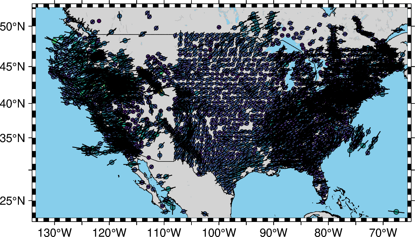
Finally, we can plot the measurements using the plot_splitting_map function defined below.
plot_splitting_map(dfselected, boxcoordinates=[
                   minlon, maxlon, minlat, maxlat], dcoord=0.5, dtscale=0.2, penwidth="0.5p",
                   proj="M10c", figname='splitting_map.png', frame=["a5f1", "WSen"],
                   markersizescale=0.1)
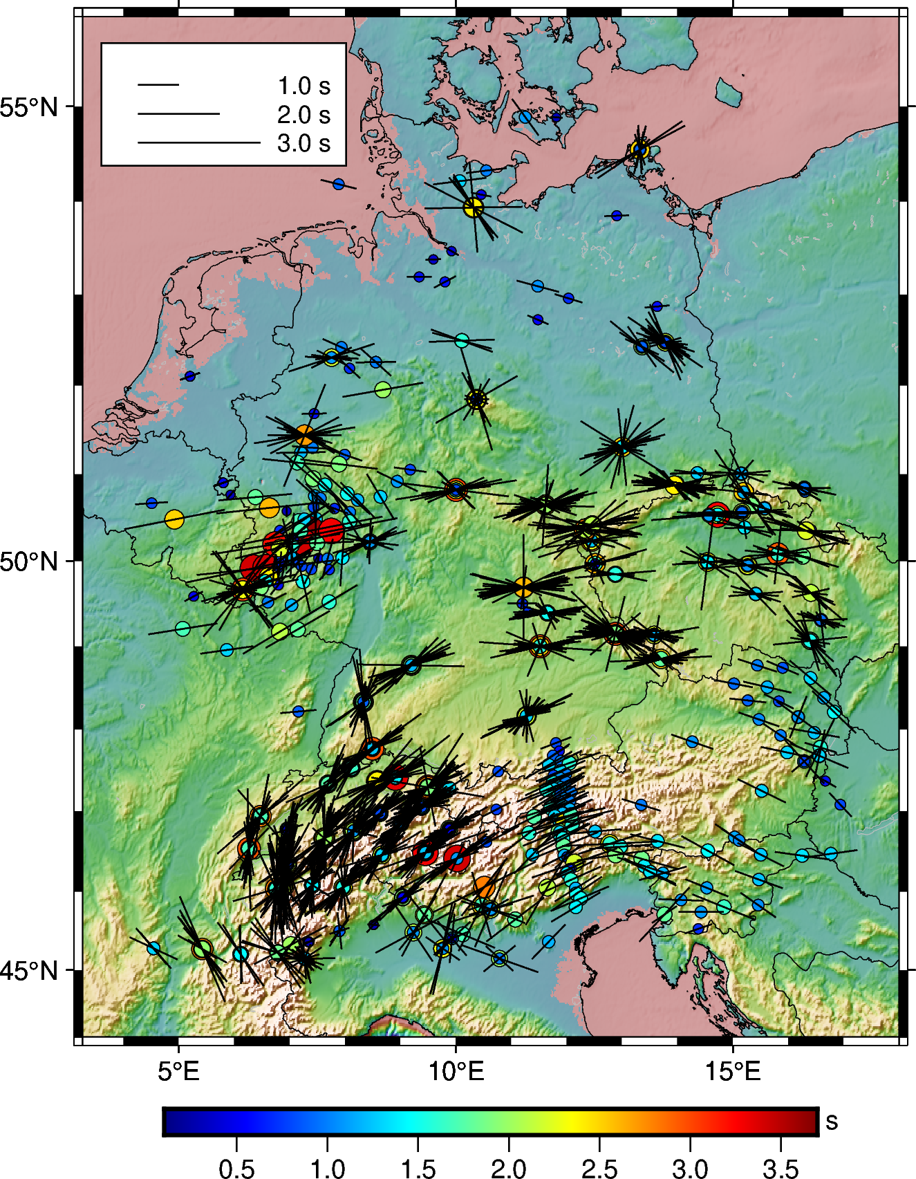
Topographic splitting map of Germany
# germany
minlon, maxlon = 4.26, 17.00
minlat, maxlat = 45.14, 54.92
dftmp1 = df[(minlon < df['Longitude']) & (df['Longitude'] < maxlon)]
dfselected = dftmp1[(minlat < df['Latitude']) & (df['Latitude'] < maxlat)]
dfselected.reset_index(inplace=True)
plot_splitting_map(dfselected, boxcoordinates=[
                minlon, maxlon, minlat, maxlat], dcoord=0.5, dtscale=0.5, penwidth="0.5p",
                proj="M10c", figname='splitting_map.png', frame=["a5f1", "WSen"],
                markersizescale=0.1, colormap="topo", markercolormap="jet")
Shear-wave splitting function
If the gist’s PyGMT calls throw a fill/color error, this is why. PyGMT renamed the color= argument of fig.plot(...) to fill= (deprecated in v0.8, later removed). On a current PyGMT, replace any color= in the plotting function with fill=. The behavior is unchanged — only the keyword differs.
Recap
- Two numbers per station. Shear-wave splitting reports φ (fast-axis azimuth) and δt (fast–slow delay time); together they probe upper-mantle anisotropy.
- The map is a field of bars. Each measurement is drawn as a bar: orientation = φ, length ∝ δt — so patterns in bar direction reveal regional anisotropy.
- Read the database with pandas. The Montpellier
splittingDB.txtis pipe-delimited Latin-1; coercephi/dtto numeric and filter by a lon/lat box to select your region. - PyGMT draws the rest. A helper (
plot_splitting_map) places the bars over a plain or topographic basemap; rememberfill=replacedcolor=in modern PyGMT.
Where to go next
- Montpellier shear-wave splitting database: splitting.gm.univ-montp2.fr/DB
- PyGMT
fig.plotdocs: pygmt.org/latest/api/generated/pygmt.Figure.plot.html - The plotting helper (gist): gist.github.com/earthinversion/cc72c744332691e3e5bba707372f6ca9
References
Kumar, U., & Legendre, C. P. (2021). STADIUM-Py: Python command-line interface for automated receiver functions and shear-wave splitting measurements (Version 1.0) [Computer software]. Zenodo. https://doi.org/10.5281/zenodo.4686103
Kumar, U., Legendre, C. P., & Huang, B. S. (2021). Crustal structure and upper mantle anisotropy of the Afar triple junction. Earth, Planets and Space, 73(1), Article 166. https://doi.org/10.1186/s40623-021-01495-0
Wüstefeld, A., Bokelmann, G. H. R., Barruol, G., & Montagner, J.-P. (2009). Identifying global seismic anisotropy patterns by correlating shear-wave splitting and surface-wave data. Physics of the Earth and Planetary Interiors, 176(3–4), 198–212. https://doi.org/10.1016/j.pepi.2009.05.006
Resources
Found this article useful?
Loading likes…
Disclaimer of liability
The information provided by the Earth Inversion is made available for educational purposes only.
Whilst we endeavor to keep the information up-to-date and correct. Earth Inversion makes no representations or warranties of any kind, express or implied about the completeness, accuracy, reliability, suitability or availability with respect to the website or the information, products, services or related graphics content on the website for any purpose.
UNDER NO CIRCUMSTANCE SHALL WE HAVE ANY LIABILITY TO YOU FOR ANY LOSS OR DAMAGE OF ANY KIND INCURRED AS A RESULT OF THE USE OF THE SITE OR RELIANCE ON ANY INFORMATION PROVIDED ON THE SITE. ANY RELIANCE YOU PLACED ON SUCH MATERIAL IS THEREFORE STRICTLY AT YOUR OWN RISK.
Leave a comment