Automatic P/S Phase Picking with Deep Learning Using SeisBench

Seven years ago today, on 6 July 2019, the Ridgecrest M7.1 earthquake struck eastern California. If you had a seismogram of it on your laptop, how would you mark exactly when the P-wave and the S-wave arrived? The classic answer is a hand-tuned energy detector like STA/LTA. The modern answer is a neural network that learned the shape of an arrival from millions of analyst-labeled examples — and thanks to SeisBench, you can run one on your own data in about ten lines of Python, with no training required.

This post is the hands-on companion to Modern Seismic Monitoring Systems, which lays out why ML has taken over earthquake monitoring. Here we do the first stage of that pipeline for real: load a waveform with ObsPy, run a pre-trained PhaseNet picker, and plot the P and S picks.

The workflow at a glance

The whole tutorial is four boxes:

Setup

SeisBench installs from PyPI and pulls in PyTorch and ObsPy for you:

pip install seisbench obspy matplotlib

Step 1 — Load a waveform with ObsPy

We pull the three broadband components (HH? → HHE, HHN, HHZ) for the Ridgecrest mainshock from station CI.GSC (Goldstone), about 90 km from the epicenter — far enough that the P and S arrivals are clearly separated. If ObsPy Stream and Client objects are new to you, start with Getting started with ObsPy.

from obspy import UTCDateTime
from obspy.clients.fdsn import Client

client = Client("SCEDC")                      # Southern California data center
origin = UTCDateTime("2019-07-06T03:19:53")   # Ridgecrest M7.1 mainshock

stream = client.get_waveforms(
    network="CI", station="GSC", location="*", channel="HH?",
    starttime=origin - 10, endtime=origin + 120,
)
stream.detrend("linear")                       # light prep; the model does the rest
print(stream)

3 Trace(s) in Stream:
CI.GSC..HHE | 2019-07-06T03:19:42.998300Z - ... | 100.0 Hz, 13001 samples
CI.GSC..HHN | 2019-07-06T03:19:42.998300Z - ... | 100.0 Hz, 13001 samples
CI.GSC..HHZ | 2019-07-06T03:19:42.998300Z - ... | 100.0 Hz, 13001 samples

Three components, sampled at 100 Hz. That’s exactly the diet PhaseNet was trained on.

Step 2 — Load a pre-trained model

This is the line that would otherwise be a research project. from_pretrained downloads a set of learned weights and returns a ready-to-run network:

import seisbench.models as sbm

model = sbm.PhaseNet.from_pretrained("stead")   # trained on the global STEAD dataset
model.eval()                                     # inference mode

The "stead" string names the weight set, not the architecture. Different groups have trained PhaseNet on different regions and datasets, and the choice matters (more on that in the gotchas). List every option that ships with SeisBench:

print(sbm.PhaseNet.list_pretrained(details=True))

Step 3 — annotate(): continuous probability curves

The lowest-level output is annotate, which slides the network across your waveform and returns a new Stream of probability traces — one each for P, S, and noise:

preds = model.annotate(stream)
print(preds)

3 Trace(s) in Stream:
CI.GSC..PhaseNet_P | ... | 100.0 Hz, 12501 samples
CI.GSC..PhaseNet_S | ... | 100.0 Hz, 12501 samples
CI.GSC..PhaseNet_N | ... | 100.0 Hz, 12501 samples

Each sample of PhaseNet_P is the model’s probability, from 0 to 1, that a P arrival is happening at that instant. Plot the waveform above these curves and the picks jump out as sharp spikes:

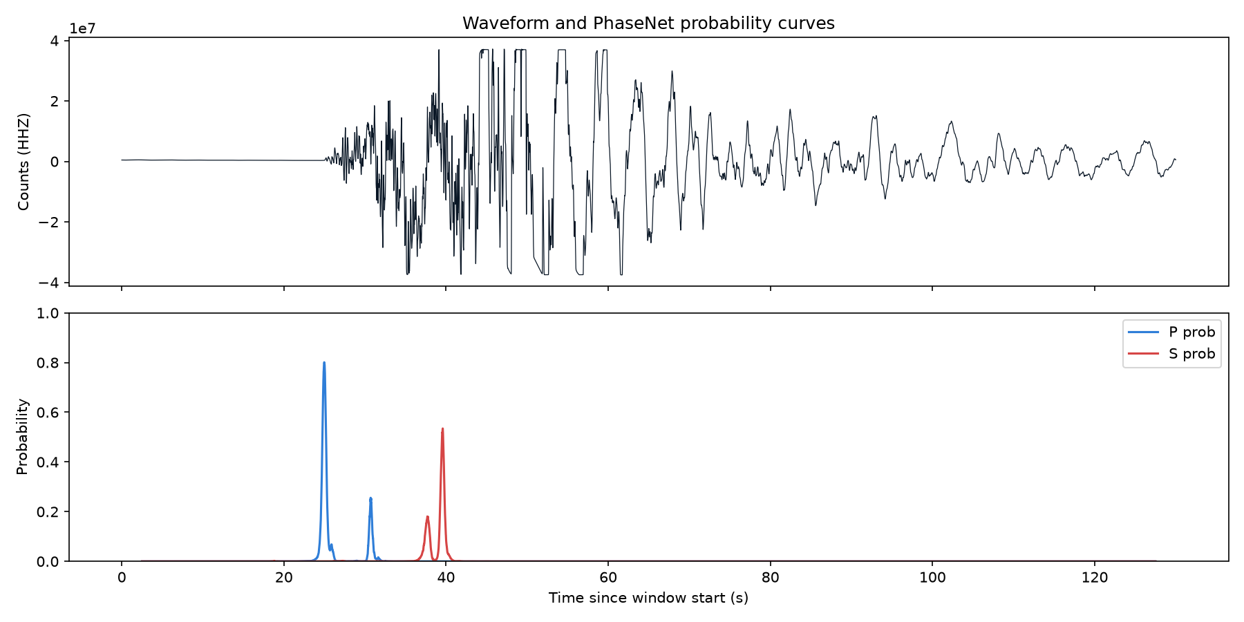
Notice there’s no thresholding yet — just smooth probability. Turning those curves into a short list of arrivals is the next step.

Step 4 — classify(): discrete picks

classify runs annotate under the hood, then finds and thresholds the peaks to return a tidy list of picks:

out = model.classify(stream)
for pick in out.picks:
    print(pick.trace_id, pick.phase, pick.peak_time, round(pick.peak_value, 2))

CI.GSC. P 2019-07-06T03:20:07.968300Z 0.8
CI.GSC. S 2019-07-06T03:20:22.588300Z 0.53

There they are: a P pick at 03:20:07.97 with confidence 0.80, and an S pick at 03:20:22.59 with confidence 0.53. The two arrivals sit 14.6 s apart — the S − P time — comfortably resolved at this ~90 km regional distance. Each pick is an object with .trace_id, .peak_time, .peak_value, and .phase, so the whole result drops straight into a table:

out.picks.to_dataframe().to_csv("picks.csv", index=False)

out = model.classify(stream, P_threshold=0.2, S_threshold=0.2)
print(out.picks.to_dataframe()[["phase", "time", "probability"]])

Step 5 — Plot the picks on the seismogram

Finally, draw the picks as vertical lines on the raw waveform — the figure you’d actually put in a report:

import matplotlib.pyplot as plt

z = stream.select(channel="HHZ")[0]
t0 = z.stats.starttime
colors = {"P": "#2f7ed8", "S": "#d64545"}

fig, ax = plt.subplots(figsize=(12, 4))
ax.plot(z.times(), z.data, color="#0a1726", lw=0.6)
for pick in out.picks:
    ax.axvline(pick.peak_time - t0, color=colors[pick.phase], lw=1.8, label=f"{pick.phase} pick")
ax.set_xlabel("Time since window start (s)")
ax.legend()
fig.tight_layout()

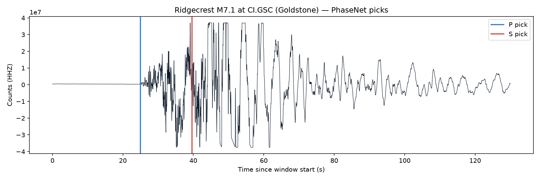
That’s the full loop — from a raw FDSN request to labeled P and S arrivals — in one short script.

Swap in EQTransformer with one line

Because every SeisBench picker shares the same annotate / classify interface, changing models is a one-line edit. EQTransformer is an attention-based network that does event detection and P/S picking together:

eqt = sbm.EQTransformer.from_pretrained("original")
eqt_out = eqt.classify(stream)

eqt_out.picks reads exactly like PhaseNet’s, and eqt_out.detections adds the time windows where EQTransformer thinks an event is present. On this record it flags the event and picks the P; nudge its pick thresholds if you want the S as well. Being able to swap PhaseNet for EQTransformer and benchmark them on your data with no other code change is the whole point of a common framework.

Gotchas worth knowing

Where to go next

• The SeisBench documentation and GitHub repo — model list, dataset loaders, and example notebooks.
• The big picture: Modern Seismic Monitoring Systems — how picking feeds association and location.
• What you do with picks: Probabilistic Earthquake Location with NonLinLoc turns P and S arrival times into a hypocenter.

You now have a complete, reproducible picker: point ObsPy at any station and event, pick with a state-of-the-art network, and plot the arrivals — the same first stage that modern monitoring systems run at continental scale.

References

1. SeisBench — A Toolbox for Machine Learning in Seismology — Woollam et al., 2022, Seismological Research Letters.
2. PhaseNet: A Deep-Neural-Network-Based Seismic Arrival Time Picking Method — Zhu & Beroza, 2019, Geophysical Journal International.
3. Earthquake Transformer — an attentive deep-learning model for simultaneous earthquake detection and phase picking — Mousavi et al., 2020, Nature Communications.
4. Which Picker Fits My Data? A Quantitative Evaluation of Deep Learning Based Seismic Pickers — Münchmeyer et al., 2022, JGR: Solid Earth.