Wavelet analysis applied to the real dataset in a quick and easy way (codes included)

A wavelet series represents a real or complex-valued function as a series built from a single “mother” wavelet — stretched, shifted, and scaled. The easiest way in is by contrast with the Fourier Transform: the Fourier Transform tells you which frequencies are in a signal, but not when they occur. Wavelets recover that missing “when.”

Fourier Transform

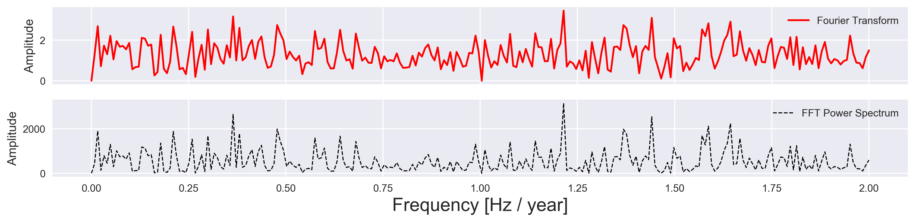
The Fourier Transform is a useful tool to transform a signal from its time domain to its frequency domain. The peaks in the frequency spectrum correspond to the most occurring frequencies in the signal. The Fourier Transform is reliable when the frequency spectrum is stationary (the frequencies present in the signal are not time-dependent). However, the Fourier Transform of the whole time series cannot tell the instant a particular frequency rises.

A quick fix is to use a sliding window to find a spectrogram that gives the information of both time and frequency (famously known as Short-time Fourier transform). However, this uses the rigid length of the window and hence limits the resolution in frequency. This is due to the uncertainty principle (duration-bandwidth theorem) in signal analysis with a tradeoff in the frequency and time resolution (Papoulis 1977; Franks 1969), similar to the Heisenberg uncertainty principle in quantum mechanics for position and momentum of a particle.

Wavelet Transform

Since in geosciences, we work mostly with dynamical systems, most of the signals are non- stationary in nature. In such cases, the Wavelet Transform is a much better approach.

The Wavelet Transform retains high resolution in both time and frequency domains (Torrence & Compo 1998; Chao et al. 2014). It tells us both the details of the frequency present in the signal along with its location in time. This is achieved by analyzing the signal at different scales. Unlike the Fourier Transform that uses a series of sine waves with different frequencies, the Wavelet Transform uses a series of functions called wavelets, each with different scales to analyze a signal. The advantage of using a wavelet is that wavelets are localized in time unlike their counterparts in the Fourier Transform. This property of time localization of wavelets can be exploited by multiplying the signal with wavelets at different locations in time, starting from the beginning and slowly moving towards the end of the signal. This procedure is known as convolution. We can iterate the whole process by increasing the scale of the wavelet at each iteration. This will give us the wavelet spectrogram (or scaleogram). The scales are analogous to the frequency in the Fourier Transform. The scales can be converted to the pseudo-frequencies by the relation:

where $f_{\alpha}$ is the pseudo-frequency, $f_{c}$ is the central frequency of the mother wavelet and $\alpha$ is the scaling factor. This relation shows that the higher scale factor (longer wavelet) corresponds to a smaller frequency. Hence, scaling the wavelet in the time domain can be used to analyze smaller frequencies in the frequency domain.

Wavelet Analysis applied on El Niño–Southern Oscillation sea surface temperature & Indian monsoon rainfall dataset

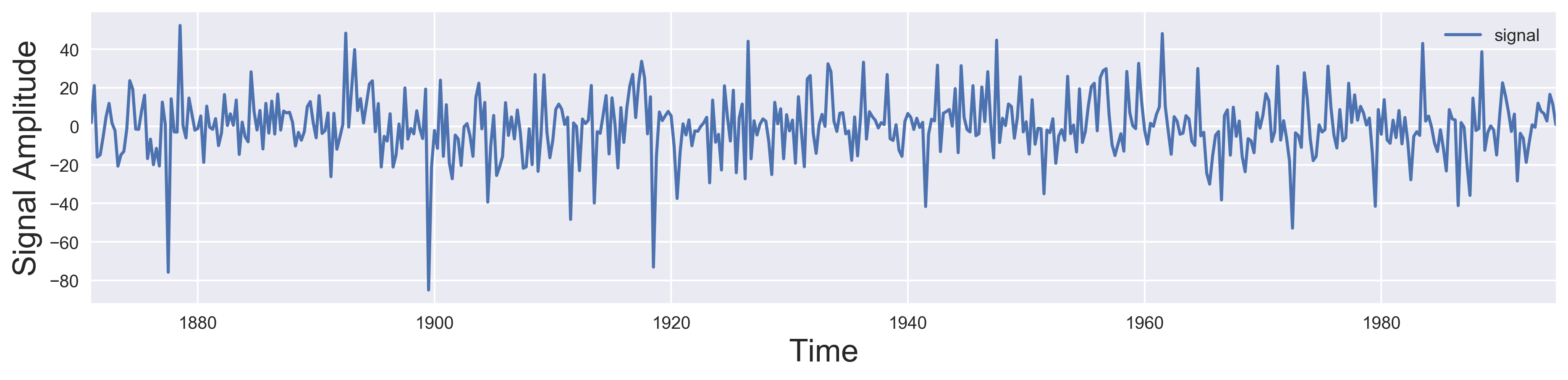
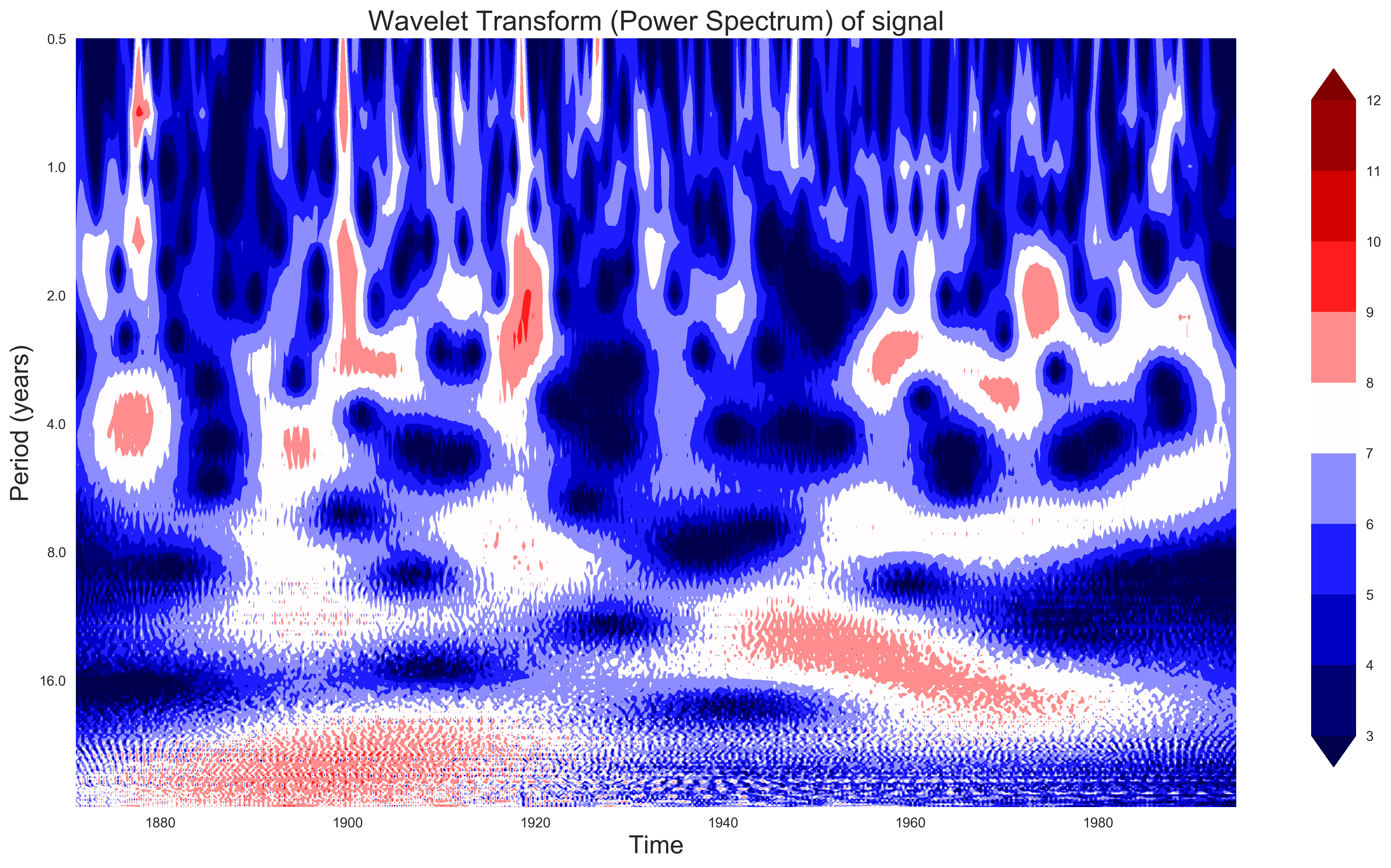
I apply the Wavelet analysis concept on the quarterly dataset for El Niño–Southern Oscillation (ENSO) sea surface temperature in degree Celsius (1871-1997) and Indian monsoon rainfall in mm (1871-1995) (Torrence & Webster 1999). The color pattern in the wavelet spectrogram is taken as log2(power). The wavelet used for this analysis is the complex Morlet wavelet with bandwidth 1.5 and normalized center frequency of 1.0. If the scale is too low, then aliasing due to the violation of Nyquist frequency may occur. If the scale is too large, the wavelet computation maybe is computationally intensive.

import pywt
import numpy as np
import matplotlib.pyplot as plt
import pandas as pd
plt.style.use('seaborn')

dataset = "monsoon.txt"
df_nino = pd.read_table(dataset, skiprows=19, header=None)

N = df_nino.shape[0]
t0 = 1871
dt = 0.25
time = np.arange(0, N) * dt + t0

signal = df_nino.values.squeeze() #to get the scalar values
signal = signal - np.mean(signal)

scales = np.arange(1, 128) #set the wavelet scales

def plot_signal(time, signal, average_over=5, figname=None):
    fig, ax = plt.subplots(figsize=(15, 3))
    ax.plot(time, signal, label='signal')
    ax.set_xlim([time[0], time[-1]])
    ax.set_ylabel('Signal Amplitude', fontsize=18)
    # ax.set_title('Signal + Time Average', fontsize=18)
    ax.set_xlabel('Time', fontsize=18)
    ax.legend()
    if not figname:
        plt.savefig('signal_plot.png', dpi=300, bbox_inches='tight')
    else:
        plt.savefig(figname, dpi=300, bbox_inches='tight')
    plt.close('all')

plot_signal(time, signal) #plot and label the axis

Heads-up on the plot style. plt.style.use('seaborn') was removed in matplotlib 3.8 (the bare seaborn style names were deprecated in 3.6). On a current install, use the renamed style plt.style.use('seaborn-v0_8'), or call import seaborn as sns; sns.set_theme() if you have seaborn installed. Everything else in this code — pywt.cwt, np.fft.fft, and the pandas reader — is still current.

In the above code, I used the pandas read_table method to read the data in the monsoon.txt I’m not sure where I originally obtained the monsoon dataset, so I cannot cite the source. If anyone knows, please comment below. The above script uses the module wavelet_visualize for computing and plotting the figure below.

def get_fft_values(y_values, T, N, f_s):
    f_values = np.linspace(0.0, 1.0/(2.0*T), N//2)
    fft_values_ = np.fft.fft(y_values)
    fft_values = 2.0/N * np.abs(fft_values_[0:N//2])
    return f_values, fft_values

def plot_fft_plus_power(time, signal, figname=None):
    dt = time[1] - time[0]
    N = len(signal)
    fs = 1/dt
    fig, ax = plt.subplots(2, 1, figsize=(15, 3), sharex=True)
    variance = np.std(signal)**2
    f_values, fft_values = get_fft_values(signal, dt, N, fs)
    fft_power = variance * abs(fft_values) ** 2  # FFT power spectrum
    ax[0].plot(f_values, fft_values, 'r-', label='Fourier Transform')
    ax[1].plot(f_values, fft_power, 'k--',
               linewidth=1, label='FFT Power Spectrum')
    ax[1].set_xlabel('Frequency [Hz / year]', fontsize=18)
    ax[1].set_ylabel('Amplitude', fontsize=12)
    ax[0].set_ylabel('Amplitude', fontsize=12)
    ax[0].legend()
    ax[1].legend()
    # plt.subplots_adjust(hspace=0.5)
    if not figname:
        plt.savefig('fft_plus_power.png', dpi=300, bbox_inches='tight')
    else:
        plt.savefig(figname, dpi=300, bbox_inches='tight')
    plt.close('all')

plot_fft_plus_power(time, signal)

def plot_wavelet(time, signal, scales, waveletname='cmor1.5-1.0', cmap=plt.cm.seismic, title='Wavelet Transform (Power Spectrum) of signal', ylabel='Period (years)', xlabel='Time', figname=None):
    dt = time[1] - time[0]
    [coefficients, frequencies] = pywt.cwt(signal, scales, waveletname, dt)
    power = (abs(coefficients)) ** 2
    period = 1. / frequencies

    scale0 = 8
    numlevels = 10

    levels = [scale0]
    for ll in range(1, numlevels):
        scale0 *= 2
        levels.append(scale0)

    contourlevels = np.log2(levels)
    fig, ax = plt.subplots(figsize=(15, 10))
    im = ax.contourf(time, np.log2(period), np.log2(power),
                     contourlevels, extend='both', cmap=cmap)
    ax.set_title(title, fontsize=20)
    ax.set_ylabel(ylabel, fontsize=18)
    ax.set_xlabel(xlabel, fontsize=18)
    yticks = 2**np.arange(np.ceil(np.log2(period.min())),
                          np.ceil(np.log2(period.max())))
    ax.set_yticks(np.log2(yticks))
    ax.set_yticklabels(yticks)
    ax.invert_yaxis()
    ylim = ax.get_ylim()
    ax.set_ylim(ylim[0], -1)
    cbar_ax = fig.add_axes([0.95, 0.15, 0.03, 0.7])
    fig.colorbar(im, cax=cbar_ax, orientation="vertical")
    if not figname:
        plt.savefig('wavelet_{}.png'.format(waveletname),
                    dpi=300, bbox_inches='tight')
    else:
        plt.savefig(figname, dpi=300, bbox_inches='tight')
    plt.close('all')

plot_wavelet(time, signal, scales)

Which CWT to use in 2026. This post uses pywt.cwt from PyWavelets, and that is still the recommended choice. If you have seen older tutorials call scipy.signal.cwt with scipy.signal.ricker, note that both were deprecated in SciPy 1.12 and removed in SciPy 1.15 — the SciPy docs now point you to PyWavelets. So the code above is already the current, maintained path; no change needed. The complex Morlet wavelet is written cmor1.5-1.0 (bandwidth 1.5, center frequency 1.0) in PyWavelets’ naming.

Final Result

For the analysis of the ENSO dataset [Figure below (a-d)], we see that most of the power is concentrated in a 2 to 8 year period (or 0.125-0.5 Hz). We can see that up to the year 1920, there were high fluctuations in power, while there were not so much after that. We can also see that there is a shift from longer to shorter periods as time progresses. For the Indian monsoon dataset [Figure below (e-h)], although the power is evenly distributed across different periods, there is also a slight shift in power from longer periods to shorter periods as time progresses. Thus, the Wavelet Transform helps in visualizing this kind of dynamic behavior of the signals.

Recap

• The Fourier Transform answers which frequencies are present but not when — it assumes the signal is stationary. Most geophysical signals are not.
• A spectrogram (short-time Fourier transform) adds time, but a fixed window forces a rigid trade-off between time and frequency resolution.
• The wavelet transform analyzes the signal at many scales, keeping good resolution in both time and frequency. Its output is a scalogram: power over time × period.
• Scale and frequency are inversely related: $f_{\alpha} = f_c / \alpha$. Large scale ⇒ long period ⇒ low frequency.
• In Python, pywt.cwt (PyWavelets) is the current, maintained CWT — SciPy’s scipy.signal.cwt/ricker were removed in 1.15.
• Reading the ENSO and Indian-monsoon scalograms, the power sits mostly in the 2–8 year band and drifts from longer to shorter periods over time — exactly the dynamic behavior the FFT alone would hide.

Where to go next

• Wavelet transform: towards multi-resolution analysis — the theory behind scales and the mother wavelet.
• Signal denoising using the Fast Fourier Transform — the Fourier baseline this post builds on.
• Concatenating daily seismic traces and plotting a spectrogram — the STFT approach for comparison.
• PyWavelets cwt reference — full list of continuous wavelets and their parameters.

References

This code was written for the purpose of the analysis in (1). If you use this code for publications, please cite (1).

1. Kumar, U., Chao, B. F., & Chang, E. T.-Y. (2020). What Causes the Common‐Mode Error in Array GPS Displacement Fields: Case Study for Taiwan in Relation to Atmospheric Mass Loading. Earth and Space Science, 7(7), e2020EA001159.
2. Chao, B. F., Chung, W., Shih, Z., & Hsieh, Y. (2014). Earth’s rotation variations: A wavelet analysis. Terra Nova, 26(4), 260–264.
3. Franks, L. E. (1969). Signal theory. Prentice-Hall. (No DOI — book.)
4. Papoulis, A. (1977). Signal analysis (Vol. 191). McGraw-Hill, New York. (No DOI — book.)
5. Torrence, C., & Compo, G. P. (1998). A practical guide to wavelet analysis. Bulletin of the American Meteorological Society, 79(1), 61–78.
6. Wavelet transform (Wikipedia)