Introduction
In this post, we will walk through the process of creating a clipped relief map in Python. This technique is particularly useful for visualizing topographic data within specific geographic boundaries, such as coastlines. If you’re interested in plotting geospatial data clipped by coastlines, you can refer to our previous post here.
In this tutorial, we’ll apply a similar approach, but instead of a general geospatial dataset, we will use a 1-arc minute topographic map, which we also employed in a previous post. This allows us to generate a visually compelling map that highlights the relief of the land while masking out regions outside the coastlines.
To achieve this, we’ll leverage the Path module from matplotlib to work with the polylines representing the coastline of Taiwan. The concept is straightforward—though it may not be the most computationally efficient. We first plot the topography on the map, select the coastal polylines using Path, and then mask the regions outside the coastline with a specified color, such as light blue for the sea.
Creating a Clipped Relief Map: Step by Step
Step 1: Setting Up the Basemap
We start by importing the necessary libraries, including Basemap from mpl_toolkits.basemap, matplotlib, and netCDF4 for handling gridded datasets like ETOPO1. This dataset provides global topography data at a 1-arc minute resolution, which we will use for our map.
from mpl_toolkits.basemap import Basemap
import matplotlib.pyplot as plt
import numpy as np
import netCDF4
from matplotlib.colors import LightSource
from matplotlib.patches import Path, PathPatch

etopo_file = "/Users/utpalkumar50/Documents/bin/ETOPO1_Bed_g_gmt4.grd"

lonmin, lonmax = 119.5, 122.5
latmin, latmax = 21.5, 25.5

fig, ax = plt.subplots(figsize=(10, 10))
map = Basemap(projection='merc', resolution='f', area_thresh=10000.,
              llcrnrlon=lonmin, llcrnrlat=latmin, urcrnrlon=lonmax, urcrnrlat=latmax)
Step 2: Loading and Preparing the Topographic Data
Next, we load the ETOPO1 data and extract the relevant sections based on our specified latitude and longitude ranges. The data is then sliced to focus on the region around Taiwan.
f = netCDF4.Dataset(etopo_file)
lons = f.variables['lon'][:]
lats = f.variables['lat'][:]
etopo = f.variables['z'][:]

lonmin, lonmax = lonmin - 1, lonmax + 1
latmin, latmax = latmin - 1, latmax + 1

lons_col_index = np.where((lons > lonmin) & (lons < lonmax))[0]
lats_col_index = np.where((lats > latmin) & (lats < latmax))[0]

etopo_sl = etopo[lats_col_index[0]:lats_col_index[-1]+1, lons_col_index[0]:lons_col_index[-1]+1]
lons_sl, lats_sl = np.meshgrid(lons[lons_col_index], lats[lats_col_index])
Step 3: Shading the Relief Map
To create a visually appealing relief map, we use LightSource to add shading, which enhances the three-dimensional appearance of the topography.
ls = LightSource(azdeg=315, altdeg=45)
rgb = ls.shade(np.array(etopo_sl), cmap=plt.cm.terrain, vert_exag=1, blend_mode='soft')

map.imshow(rgb, zorder=2, alpha=0.8, cmap=plt.cm.terrain, interpolation='bilinear')
map.drawcoastlines(color='k', linewidth=1, zorder=3)
map.drawcountries(color='k', linewidth=1, zorder=3)
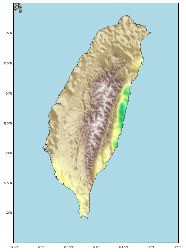
Step 4: Masking the Regions Outside the Coastline
To highlight the land features within Taiwan while masking out the surrounding sea, we create a PathPatch using the coastline polygons. The patch is then added to the plot, effectively hiding the regions outside the specified boundaries.
x0, x1 = ax.get_xlim()
y0, y1 = ax.get_ylim()
map_edges = np.array([[x0, y0], [x1, y0], [x1, y1], [x0, y1]])
polys = [p.boundary for p in map.landpolygons]
polys = [map_edges] + polys[:]
codes = [[Path.MOVETO] + [Path.LINETO for _ in p[1:]] for p in polys]
verts = [v for p in polys for v in p]
codes = [code for cs in codes for code in cs]

path = Path(verts, codes)
patch = PathPatch(path, facecolor='lightblue', edgecolor='none', zorder=4)

ax.add_patch(patch)
plt.savefig('station_map_masked.png', bbox_inches='tight', dpi=300)
plt.close('all')
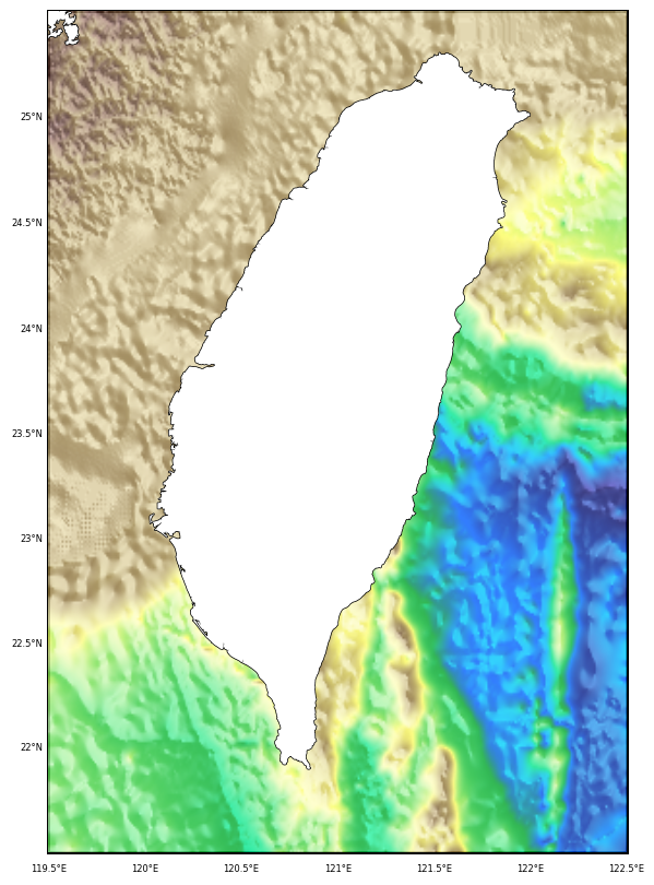
Step 5: Reversing the Mask
It’s also possible to reverse the masking, keeping the bathymetric features of the sea while masking out the land regions. This can be done by adjusting the facecolor in the PathPatch.
# Reuse previous code with a slight modification in PathPatch facecolor
patch = PathPatch(path, facecolor='white', edgecolor='none', zorder=4)
ax.add_patch(patch)

plt.savefig('station_map_masked_reverse.png', bbox_inches='tight', dpi=300)
plt.close('all')
Conclusion
In this post, we’ve demonstrated how to generate a clipped relief map using Python, focusing on topographic data within the coastlines of Taiwan. This method, while simple, is a powerful tool for creating focused visualizations of geographic regions. Whether you’re interested in highlighting land features or bathymetric data, the matplotlib and Basemap libraries provide robust capabilities for geospatial analysis and visualization.
For further exploration, you can download the complete code here.