Monte Carlo Simulation for Correlation Testing: Python and MATLAB Implementations

Overview

Monte Carlo Simulations (MCS) are powerful tools used to assess statistical properties that are otherwise difficult to evaluate. In this article, we explore how MCS can be employed to test the significance of the correlation between two datasets. We will demonstrate this using both Python and MATLAB, providing detailed explanations and code examples.

Introduction to Monte Carlo Simulations

Monte Carlo Simulation studies involve generating random sample data based on predefined parameters, such as population means and standard deviations, and then repeatedly analyzing these data to assess the behavior of statistics of interest under various conditions (e.g., sample size, variability). This method is especially useful for estimating the distribution of a statistic and its confidence intervals.

What is Monte Carlo Simulation?

MCS studies are computer-driven experimental investigations in which certain parameters, such as population means and standard deviations that are known a priori, are used to generate random (but plausible) sample data (Mooney 1997). These generated data are then used to evaluate the sampling behavior of one or more statistics of interest. This process of generating and analyzing data is repeated over many iterations and differing conditions that are thought to influence the sampling behavior of the statistic of interest (e.g., through increasing sample size, mean differences, variability). 3

Python Implementation

Let’s start with a Python implementation of Monte Carlo Simulation to test for the correlation between two datasets.

import numpy as np
import matplotlib.pyplot as plt

# Parameters
num_sim = 10000  # Number of simulations
sample_size = 50  # Number of data points in each sample

# Pre-allocate the results vector
results = np.zeros(num_sim)

# Run simulations
for i in range(num_sim):
    # Draw two sets of random numbers from the normal distribution
    data = (np.random.randn(sample_size, 2) ** 2) * 10 + 20
    
    # Compute the correlation between the two sets of numbers
    results[i] = np.corrcoef(data[:, 0], data[:, 1])[0, 1]

# Visualize the results
plt.hist(results, bins=100, color='blue', alpha=0.75)
plt.xlabel('Correlation value')
plt.ylabel('Frequency')
plt.title('Monte Carlo Simulation of Correlation Coefficients')

# Calculate the 95th percentile for significance
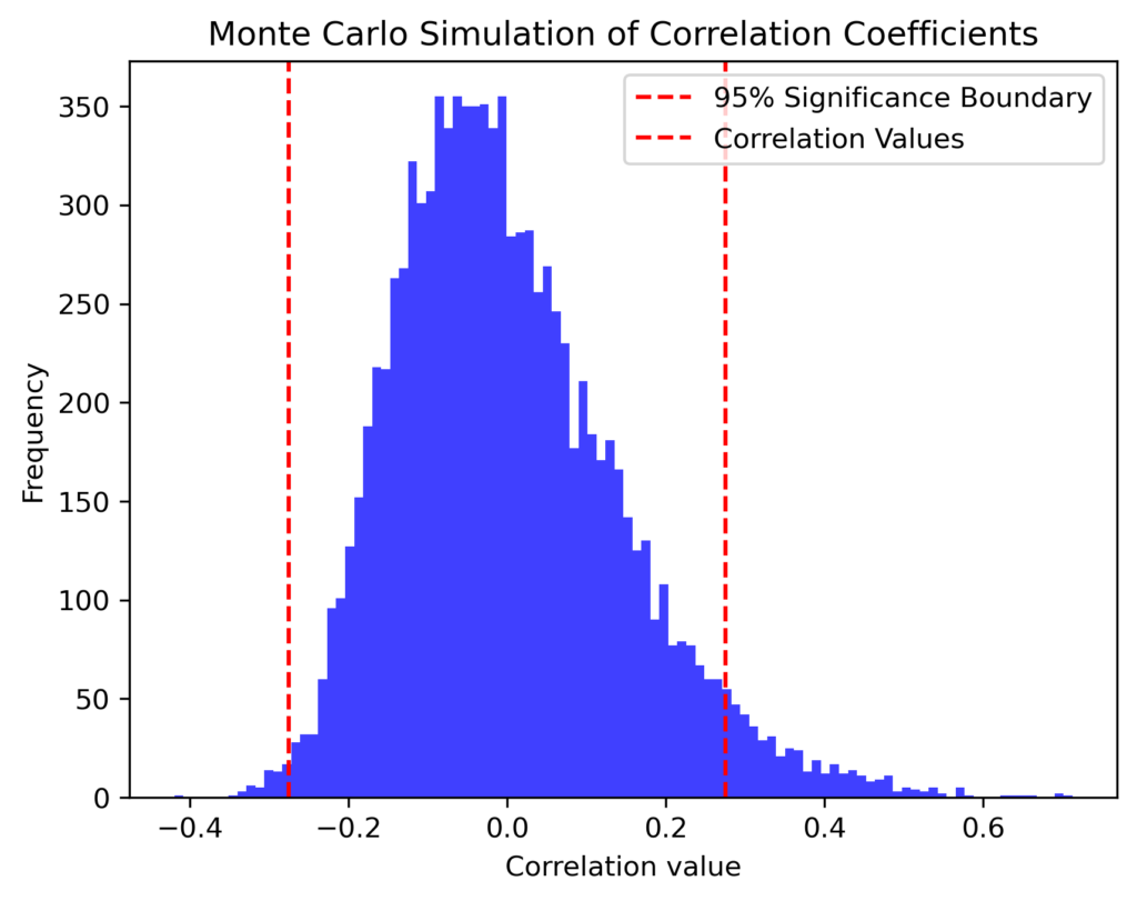
val = np.percentile(np.abs(results), 95)
plt.axvline(val, color='red', linestyle='--')
plt.axvline(-val, color='red', linestyle='--')
plt.legend(['95% Significance Boundary', 'Correlation Values'])

plt.show()

# Output the 95th percentile value
print(f"The central 95% of correlation values lie between +/- {val:.4f}")

Results

In the Python implementation, we ran 10,000 simulations, calculating the correlation between two randomly generated datasets for each simulation. The distribution of these correlation coefficients is plotted, and the 95th percentile is highlighted to indicate the range within which most correlation values lie. This range can be used to assess the significance of observed correlations in real datasets.

MATLAB Implementation

Next, let’s implement the same Monte Carlo Simulation in MATLAB.

MATLAB Code

%% Monte Carlo simulations of correlation values
clear; close all; clc;

% Define parameters
numsim = 10000;   % Number of simulations to run
samplesize = 50;  % Number of data points in each sample

% Pre-allocate the results vector
results = zeros(1, numsim);

% Loop over simulations
for num = 1:numsim
    % Draw two sets of random numbers, each from the normal distribution
    data = (randn(samplesize, 2).^2) * 10 + 20;

    % Compute the correlation between the two sets of numbers and store the result
    results(num) = corr(data(:, 1), data(:, 2));
end

% Visualize the results
figure; hold on;
histogram(results, 100);
xlabel('Correlation value');
ylabel('Frequency');
title('Monte Carlo Simulation of Correlation Coefficients');

% Calculate the 95th percentile for significance
val = prctile(abs(results), 95);
ax = axis;
plot([val val], ax(3:4), 'r-', 'LineWidth', 2);
plot(-[val val], ax(3:4), 'r-', 'LineWidth', 2);
legend('Correlation Values', '95% Significance Boundary');

% Display the 95th percentile value
disp(['The central 95% of correlation values lie between +/- ', num2str(val)]);

Results

In MATLAB, the approach is similar. After running 10,000 simulations, we compute the correlation coefficients and visualize their distribution. The 95th percentile is also calculated and visualized, providing a clear indication of where most correlation values fall, helping to determine the significance of any observed correlation.

Conclusion

Monte Carlo Simulations offer a flexible and intuitive approach to testing the significance of correlation coefficients between datasets. By using these simulations, we can assess the likelihood that an observed correlation is due to chance. Both Python and MATLAB provide robust tools for implementing these simulations, allowing for detailed statistical analysis.

References

1. Lectures on Statistics and Data Analysis in MATLAB
2. Assessing the Significance of the Correlation between Two Spatial Processes
3. Teaching Statistics With Monte Carlo Simulation

[zotpress items=”{9687752:MX4FWEQH}” style=”apa”]