Comparative Hypothesis Testing: Implementing Randomization with Python and MATLAB

Overview

This post demonstrates how to test the null hypothesis using randomization and bootstrapping methods. We will explore the implementation in both Python and MATLAB. The null hypothesis posits that two datasets originate from the same probability distribution. Under this hypothesis, if we aggregate and randomly divide the data into two sets, the results should be comparable to those obtained from the original datasets.

Python Implementation

Let’s begin with a Python implementation of the hypothesis test. We’ll use numpy for data generation and matplotlib for visualization.

import numpy as np
import matplotlib.pyplot as plt

# Generate random datasets
data1 = np.random.randn(100)
data2 = (np.random.randn(150)**2) * 10 + 20
all_data = np.concatenate([data1, data2])

# Null hypothesis: the two distributions are from the same population
mu1 = np.mean(data1)
mu2 = np.mean(data2)
actual_diff_mean = mu1 - mu2

# Using Randomization to test the hypothesis
num_sim = 10000
diff_means = np.zeros(num_sim)

for i in range(num_sim):
    np.random.shuffle(all_data)
    sim_data1 = all_data[:len(data1)]
    sim_data2 = all_data[len(data1):]
    diff_means[i] = np.mean(sim_data1) - np.mean(sim_data2)

# Visualization
plt.hist(diff_means, bins=100, alpha=0.75, color='blue')
plt.axvline(actual_diff_mean, color='red', linestyle='dashed', linewidth=2)
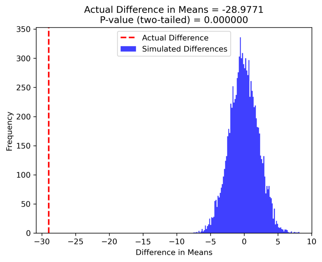
plt.title(f'Actual Difference in Means = {actual_diff_mean:.4f}\nP-value (two-tailed) = {np.mean(np.abs(diff_means) >= np.abs(actual_diff_mean)):.6f}')
plt.xlabel('Difference in Means')
plt.ylabel('Frequency')
plt.legend(['Actual Difference', 'Simulated Differences'])
plt.savefig('hypothesis_testing_python.png', dpi=300, bbox_inches='tight')

Results

In this simulation, we computed the difference in means for 10,000 random datasets and visualized the distribution of these differences. The p-value was calculated by determining the proportion of simulated differences greater than the actual observed difference.

MATLAB Implementation

Now, let’s see how to perform the same hypothesis test in MATLAB. The MATLAB implementation follows a similar approach using randomization and bootstrapping.

%% Hypothesis Testing in MATLAB
clear; close all; clc;

% Generate random datasets
data1 = randn(100, 1);
data2 = (randn(150, 1).^2) * 10 + 20;
all_data = [data1; data2];

% Null hypothesis: the two distributions are from the same population
mu1 = mean(data1);
mu2 = mean(data2);
actual_diff_mean = mu1 - mu2;

% Using Randomization to test the hypothesis
num_sim = 10000;
diff_means = zeros(1, num_sim);

for i = 1:num_sim
    indx = randperm(length(all_data));
    data_sim = all_data(indx);
    data_sim1 = data_sim(1:length(data1));
    data_sim2 = data_sim(length(data1) + 1:end);
    diff_means(i) = mean(data_sim1) - mean(data_sim2);
end

% Visualization
figure; hold on;
histogram(diff_means, 100);
ax = axis;
plot(repmat(actual_diff_mean, [1, 2]), ax(3:4), 'r-', 'LineWidth', 2);
p_val = sum(abs(diff_means) > abs(actual_diff_mean)) / length(diff_means);
title(sprintf('Actual Difference in Means = %.4f; P-value (two-tailed) = %.6f', actual_diff_mean, p_val));
legend('Simulated Differences', 'Actual Difference');
xlabel('Difference in Means');
ylabel('Frequency');
hold off;

Results

In the MATLAB implementation, we similarly generate random datasets, perform bootstrapping, and visualize the difference in means. The p-value is calculated in the same way as in the Python version.

Conclusion

Both Python and MATLAB offer robust tools for performing hypothesis testing through randomization and bootstrapping. Depending on your preference and specific requirements, you can choose either of these environments for statistical analysis. The examples provided here can be adapted to different datasets and hypothesis tests.

For further reading, see Lectures on Statistics and Data Analysis in MATLAB.