Exploring the Multi-Taper Method: A Robust Approach for Time-Frequency Analysis

Introduction

Multi-taper (MT) spectral analysis is a method that is widely used in various scientific fields, including seismology, for the time-frequency analysis of signals. This technique offers a means to assess the power spectrum of a signal in both the time and frequency domains, with the aim of reducing bias and variance in spectral estimates (see Thomson, 1982). It serves as an important tool for the spectral analysis of non-stationary signals.

Multitaper Spectrum Analysis

The multitaper algorithm shares similarities with other nonparametric spectral estimation techniques. Specifically, an -length time sequence where () is multiplied by the taper before being Fourier transformed

Unlike single-taper methods, the multitaper approach employs orthogonal tapers to refine the Power Spectral Density (PSD) estimate :

In this formulation, is a weighted average of the values, where serves as the weights designed to mitigate spectral leakage while maintaining a low variance in the estimate. The choice of weights can be guided by the eigenvalues of the tapers or through adaptive weighting, as outlined by Thomson (1982). For more advanced applications, the quadratic multitaper estimate, introduced by Prieto et al. (2007), utilizes the second derivative of the spectrum to yield a higher-resolution estimate (See Prieto et. al., 2022).

Core Concepts for Understanding the Multi-taper Spectral Analysis Method

Tapers

A taper is essentially a window function that multiplies a signal in the time domain, effectively localizing it both temporally and spectrally. The most straightforward example of a taper is a rectangular window, but there are various other types such as the Hanning or Hamming windows. In multi-taper analysis, multiple tapers are applied to the same data segment.

Slepian Functions

In multi-taper analysis, the tapers commonly employed are Slepian functions, or Discrete Prolate Spheroidal Sequences (DPSS). These are a set of orthogonal tapers optimized to minimize leakage from other frequencies during the estimation of the power spectrum.

Spectral Estimation

For each taper, the data are multiplied by the taper in the time domain, and then a Fourier transform is applied to analyze the resulting sequence in the frequency domain. These individual spectral estimates are subsequently aggregated, often by taking an average, to yield a more robust estimate of the power spectrum.

Analyze a time series to understand the concepts of Multitaper method

1. Download the MSEED data here

2. Import Python Libraries:

import numpy as np
from scipy.signal import welch
import matplotlib.pyplot as plt
from scipy.signal.windows import dpss 

3. Define DPSS parameters and generate tapers

# DPSS parameters
NW = 4.5  # Time-half bandwidth
K = 6  # Number of tapers

# Generate tapers
tapers = dpss(N, NW, K)

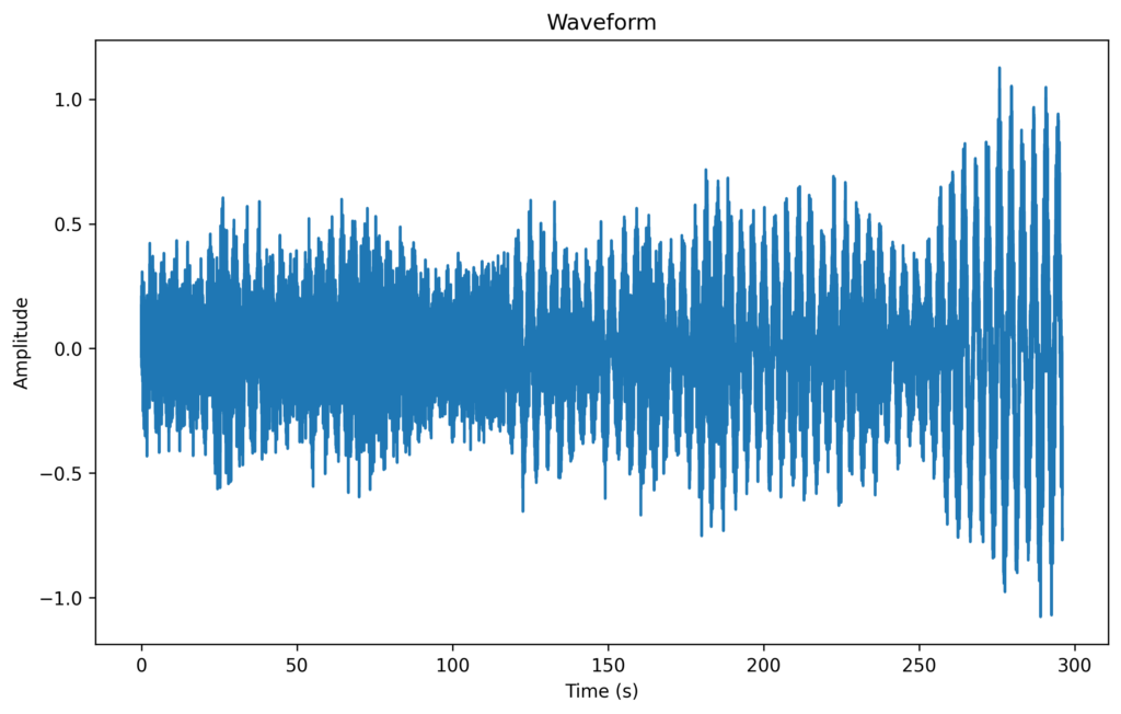
4. Visualize the trace data

from obspy import read

# Load the MSEED file
st = read("path_to_your_mseed_file.mseed")

# Extract the first trace
tr = st[0]

N = tr.stats.npts  # Number of data points
fs = tr.stats.sampling_rate  # Sampling frequency

# Time vector
t = tr.times()

noisy_signal = tr.data

fig, ax = plt.subplots(1, 1, figsize=(10, 6), sharex=True)
ax.plot(t, noisy_signal)
ax.set_xlabel('Time (s)')
ax.set_ylabel('Amplitude')
ax.set_title('Waveform')
plt.savefig("multitaper_input_waveform.png", dpi=300, bbox_inches='tight')
plt.show()

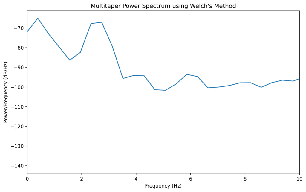
5. Apply the vanilla multitaper method on the noisy_signal

# Apply tapers
tapered_data = tapers * noisy_signal[np.newaxis, :]

# Initialize for accumulating the power spectrum
average_power_spectrum = np.zeros(N)

# Welch parameters
nperseg = 512  # Length of each segment
noverlap = 256  # Overlap between segments

# Loop over each taper
for k in range(K):
    # Apply Welch Periodogram on each tapered data
    f, Pxx = welch(tapered_data[k, :], fs, nperseg=nperseg, noverlap=noverlap)
    
    # Accumulate the power spectrum
    average_power_spectrum[:len(f)] += 10 * np.log10(Pxx)

# Average the power spectrum
average_power_spectrum[:len(f)] /= K

# Visualize
fig, ax = plt.subplots(1, 1, figsize=(10, 6), sharex=True)
ax.plot(f, average_power_spectrum[:len(f)])
ax.set_xlabel('Frequency (Hz)')
ax.set_ylabel('Power/Frequency (dB/Hz)')
ax.set_title('Multitaper Power Spectrum using Welch\'s Method')
ax.set_xlim([0, 10])
plt.savefig("multitaper_output_spectrum.png", dpi=300, bbox_inches='tight')
plt.show()

In the above script, equal weights are given to each taper but this approach will not be most efficient in practice. It is possible to decide the weights of the tapers based on its eigenvalues [tapers, eigvals = dpss(N, NW, 4, return_ratios=True)].

Implementing Thomson’s Multitaper Method

The multitaper approach previously described incorporates Welch’s method, a classical technique in spectral estimation. In this framework, multiple tapers are computed and subsequently applied to the input signal. The power spectral density (PSD) for each tapered signal is then calculated using Welch’s method. The final PSD is obtained by averaging these individual estimates, essentially forming a straightforward mean of the spectral estimates from each taper.

The “MTSpec” class available in Prieto’s Github respository extends beyond mere spectral estimates to include advanced functionalities like adaptive spectral estimation and quadratic inverse spectrum. In the adaptive spectral estimation approach, an iterative algorithm is deployed to identify optimal weightings for each taper. This algorithm ensures that the weights fall within a range of 0 to 1, thereby normalizing them.

Furthermore, Prieto’s code provides Quadratic Inversion (QI) spectral estimation specifically tailored for seismic data analysis. This method calculates the QI spectrum using the methodology proposed by Prieto et al. (2007). It is designed to mitigate the bias introduced by the curvature characteristics of the multitaper spectrum in seismic data.

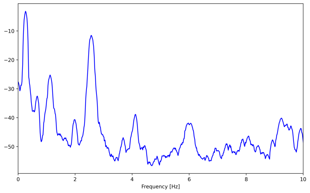
## Applying Prieto's method
import multitaper.mtspec as spec


nw = 4.5 #time-bandwidth product (twin x freq_res)/2
kspec = 6 # the standard number of tapers is calculated as K=2×NW−1. However, we could opt to use fewer tapers if computational resources are a concern.
twin = 40. #window length (time resolution is inversely proportional to freq resolution (coming from the uncertainty principle))
# Also, a shorter time window can make the spectrogram more responsive to changes in frequency content, potentially improving frequency resolution
# Decide based on how fast the data is changing
olap = 0.8 #Lower overlap may capture more dynamic changes in your signal
fmax = 25.

freq_res = (nw/twin)*2
dt = tr.stats.delta

t_vals,freq_vals,quad_vals,thomp_vals = spec.spectrogram(noisy_signal,dt,twin = twin, olap = olap, nw = nw, fmax = fmax)

max_qi_vals = np.max(quad_vals, axis=1)
log_psd_db = 10*np.log10(max_qi_vals)

fig, ax = plt.subplots(1, 1, figsize=(10, 6), sharex=True)
ax.plot(freq_vals, log_psd_db, 'b', label='Quad PSD (dB)')
ax.set_xlabel('Frequency [Hz]')
ax.set_xlim([0, 10])
plt.savefig("prieto_method_output_spectrum.png", dpi=300, bbox_inches='tight')

What are the advantages of applying MT method on a time-series data

Comparison with other methods

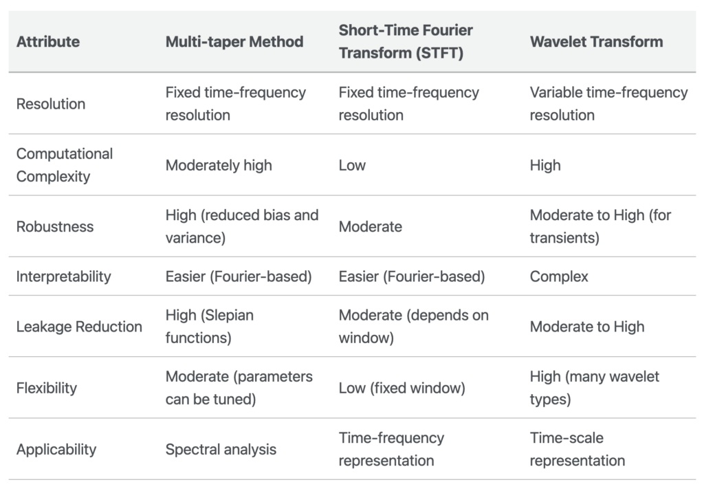
When it comes to time-frequency resolution, the Wavelet Transform has an edge, especially for non-stationary signals. Multi-taper methods offer better frequency resolution than STFT but do not have the variable resolution advantage of wavelets. However, Multi-taper methods offer robust spectral estimates, particularly in low signal-to-noise ratio scenarios, surpassing STFT in this regard. Wavelets are more suited for capturing transient phenomena rather than providing robust spectral estimates.

Conclusion

Multi-taper spectral analysis offers a robust and versatile method for time-frequency analysis. By using multiple tapers, it provides more reliable and less biased spectral estimates, which are valuable in various applications, including but not limited to seismology.

References