Introduction
Seismic tomography is an indispensable tool in the study of the Earth’s internal structure. It enables researchers to develop high-resolution models of subsurface geology, thereby facilitating our understanding of tectonic processes, resource exploration, and even earthquake hazard assessment. However, to fully grasp the complexity of the Earth’s interior, one must not only focus on the source and receiver locations but also the paths that seismic waves travel between them, often termed as “great circle paths.”
This article aims to discuss a Python-based approach to visualize great circle paths that seismic waves follow, focusing on a designated region of interest. We will utilize PyGMT (Python Generic Mapping Tools), a powerful library for creating high-quality geographical maps and plots, along with other Python libraries such as NumPy, Pandas, and Shapely for data manipulation and geometrical operations.
By the end of this article, you will have learned how to use Python code to:
- Define a specific geographic region of interest.
- Generate and plot the great circle paths between earthquake events and seismic stations.
- Filter the relevant stations based on their location and the paths that traverse the specified region.
Understanding these paths is not just an academic exercise; it is crucial for rigorous seismic tomography investigations. The generated paths can provide valuable insights into the subsurface structure below the selected region, thereby making your seismic analyses more robust and accurate.
Install PyGmt
Using python env
python -m venv geoviz
source geoviz/bin/activate
pip install pygmt
For more details, visit the article A Quick Overview on Geospatial Data Visualization using PyGMT.
Plot great-circle path traversing the region of interest
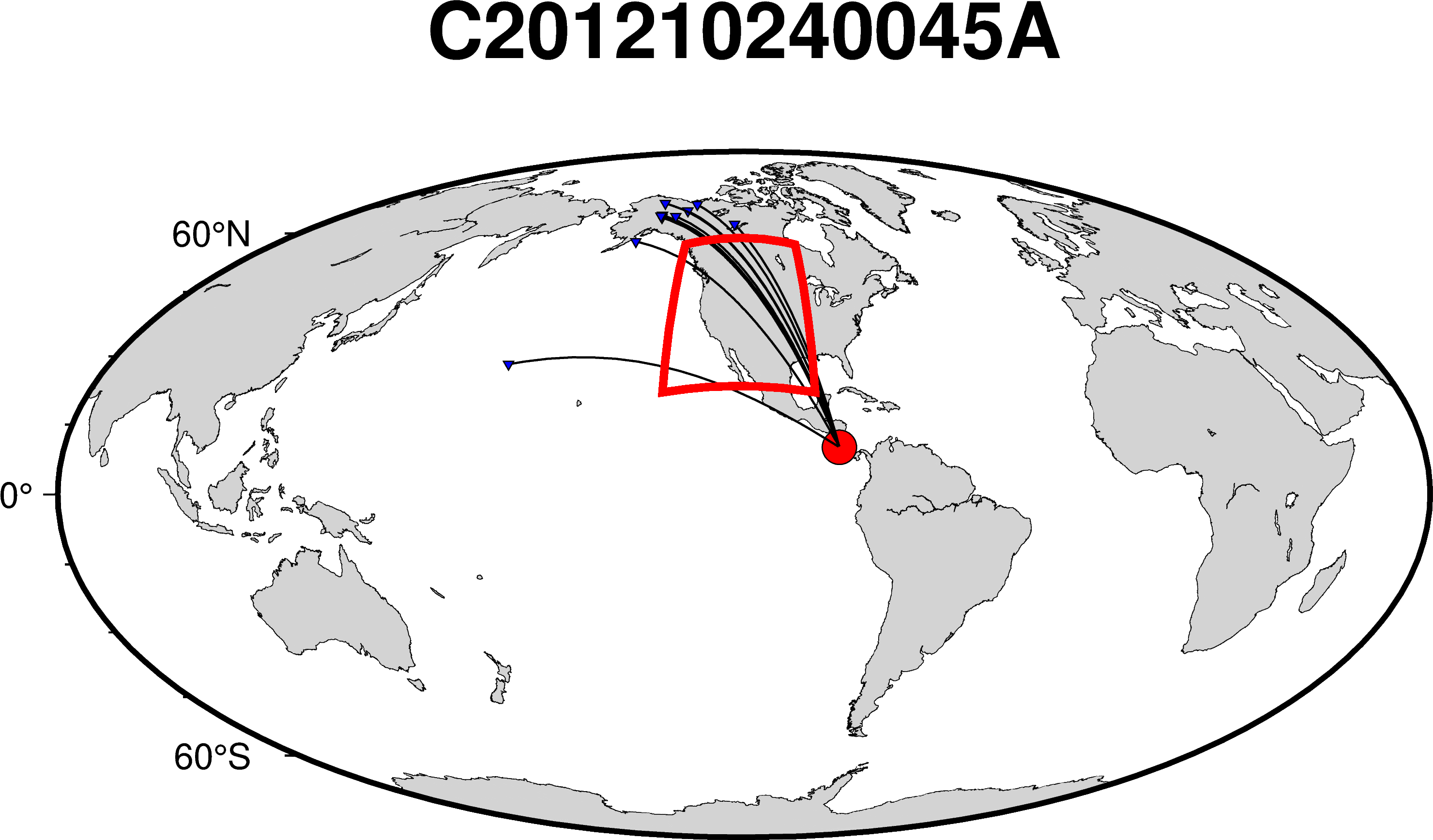
This Python script serves as a specialized tool for visualizing seismic events and their associated seismic stations within a defined geographical region. Utilizing the PyGMT library for geospatial plotting, along with data manipulation libraries like NumPy and Pandas, the script reads earthquake event and seismic station data, filters them based on their location, and plots them on a high-resolution map. It specifically highlights the great circle paths between the earthquake source and the seismic stations, aiding in seismic tomography studies by offering insights into the subsurface structure beneath the region of interest. Through the use of geometrical libraries like Shapely and geodetic calculations from Pyproj, the script efficiently determines whether these paths traverse the specified region, thereby streamlining the process of selecting relevant data for further analysis.
import pygmt
import numpy as np
import pandas as pd
import yaml, glob, os, sys
from shapely.geometry.polygon import Polygon
import pyproj
from shapely.geometry import Point


def get_region_polygon(
    # Box size
    lon_left   = -128,      # possible range: -180, 180 deg
    lon_right  = -96,      # possible range: -180, 180 deg
    lat_bottom = 27,      # possible range: -90, 90 deg
    lat_top    =  52,      # possible range: -90, 90 deg
    offset = 20, # offset in degrees from the box limits
):
    lon_left  = lon_left - offset
    lon_right = lon_right + offset
    lat_bottom = lat_bottom - offset
    lat_top = lat_top + offset

    box_lims = [[lon_left,lat_bottom], [lon_right,lat_bottom], [lon_right,lat_top], [lon_left,lat_top], [lon_left,lat_bottom]]
    box_maxdim = max(np.abs(lon_right-lon_left),np.abs(lat_top-lat_bottom))
    lims_array = np.array(box_lims)
    boxclon, boxclat = np.mean(lims_array[:, 0]),np.mean(lims_array[:, 1])
    box_polygon = Polygon(box_lims)

    return box_polygon

def is_in_domain(lon_points, lat_points, box_polygon):

    for lat, lon in zip(lat_points, lon_points):
        # print(lon, lat)
        if box_polygon.contains(Point(lon,lat)):
            return True
    return False


def main():

    ## Inversion domain
    lon_left = -128      # possible range: -180, 180 deg
    lon_right = -96      # possible range: -180, 180 deg
    lat_bottom = 27      # possible range: -90, 90 deg
    lat_top =  52      # possible range: -90, 90 deg

    ## Event info
    evbase = 'C201210240045A' # (D12O0TUA)
    evlon = -85.30
    evlat = 10.09
    evdep = 17.0
    evmag = 6.0


    ## Define polygon
    box_polygon = get_region_polygon(offset = 5)
    print("box_polygon.bounds: ",box_polygon.bounds)
    geod=pyproj.Geod(ellps="WGS84")

    out_image_station = f"{evbase}.png"

    ## plot stations
    fig = pygmt.Figure()
    projection = "W-110.5885/12c"
    fig.basemap(region='g', projection=projection, frame=["afg", f"+t{evbase}"])
    fig.coast(
        land="lightgrey",
        water="white",
        shorelines="0.1p",
        frame="WSNE",
        resolution='h',
        area_thresh=10000
    )

    if is_in_domain([evlon], [evlat], box_polygon):
        print(f"--> Skipping {evbase} because it is in domain")

    dff_event = pd.read_csv('event_station_info_D12O0TUA.txt', sep='\s+', header=None, names=['evname', 'stn', 'slon', 'slat'])
    # print(dff_event)

    assert len(dff_event) > 0, "No stations found in event_station_info_D12O0TUA.txt"

    fig.plot(x=evlon, y=evlat, style="c0.3c", color="red", pen="black")

    for stlat, stlon, sname in zip(dff_event.slat, dff_event.slon, dff_event.stn):
        if is_in_domain([stlon], [stlat], box_polygon):
            continue
        line_arc=geod.inv_intermediate(evlon,evlat,stlon,stlat,npts=300)
        lon_points=np.array(line_arc.lons)
        lat_points=np.array(line_arc.lats)
        if not is_in_domain(lon_points, lat_points, box_polygon):
            continue
        fig.plot(x=lon_points, y=lat_points, pen="0.5p,black")
        fig.plot(x=stlon, y=stlat, style="i0.1c", color="blue", pen="black")


        rectangle = [box_polygon.bounds]
        fig.plot(data=rectangle, style="r+s", pen="2p,red")

    print('----> Saving map... {}'.format(out_image_station))
    fig.savefig(out_image_station, crop=True, dpi=600)

if __name__ == "__main__":
    main()
Download the event_station_info_D12O0TUA.txt from here